Investigation 4.9: Speed It Up (cont.)

Section 21.2 Investigation 4.9: Speed It Up (cont.)

In this investigation, you will extend your consideration of paired data to tests of significance and confidence intervals.

🔗

Exercises 21.2.1 Inference for Paired Designs

Recall that student researchers wanted to compare the mean typing speed with and without up-tempo music.

🔗

\(H_0: \mu_{music} - \mu_{nomusic} = 0\) (no difference in the long run average speed)

🔗

\(H_a: \mu_{music} - \mu_{nomusic} > 0\) (on average typing speed is faster with up-tempo music)

🔗

Below are the results from the students’ paired design.

🔗

Summary statistics and dotplots for typing speeds with and without music

1. Compare to Previous Results.

Compare these results to the results in Investigation 4.8. What has changed? Will these changes impact the p-value? If so, how?

🔗

Solution.

The sample sizes are larger which would lower the p-value. The standard deviations have changed a bit but in general are similar in magnitude to before. The sample means have changed a bit, but in general are similar in magnitude to before. If anything, the difference in mean typing speed between the two groups is a bit smaller which would raise the p-value.

🔗

2. Can We Use Previous Methods?

Explain why we can’t do a randomization test or a two-sample t-test with these data.

🔗

Solution.

We don’t have "two samples." We have just one sample, the two observations are each individual should not be considered as unrelated to each other.

🔗

Key Idea.

When the data are paired (e.g., repeat observations on the same observational unit) we should not treat the two samples as independent. This ignores the information that two measurements were taken for each observational unit (we couldn’t mix up the values in the second column without altering the information in the data).

🔗

As suggested in Investigation 4.8, Question 9, we can use the differences as the response variable.

🔗

Distribution of differences in typing speeds (no music - music)

3. Distribution of Differences.

Summarize what you learn about the distribution of differences.

🔗

Solution.

The distribution of differences in typing speeds is slightly skewed to the right with a mean difference of 2.62 wpm and a standard deviation of 5.71 wpm. There are a couple of participants that performed much worse for one of the tests (\(\sim\) 10 wpm), one with the music condition and one with the no music condition.

🔗

4. Mean of Differences vs. Difference in Means.

How does the mean of the differences (\(\bar{x}_{diff}\)) compare to the difference in means (\(\bar{x}_{music} - \bar{x}_{nomusic}\))?

🔗

Equal to
Correct! \(63.588 - 66.206 = -2.62\text{,}\) the same as the mean of differences.
Greater than
Calculate the difference in means and compare.
Less than
Calculate the difference in means and compare.

🔗

5. Standard Deviation Comparison.

How does the standard deviation of the differences compare to the standard deviations of the original typing speeds in the two groups?

🔗

Greater than
Compare the SD of differences (5.71) to the original SDs (14.1 and 13.8).
Less than
Correct! The standard deviation of the differences (5.71) is much smaller than the original SDs of 14.1 and 13.8, showing the pairing was effective.
Equal to
Compare the SD of differences (5.71) to the original SDs (14.1 and 13.8).

🔗

6. Parameter and Hypotheses.

Define an appropriate parameter for investigating whether comparing typing speeds with and without music. State a null and an alternative hypothesis about this parameter.

🔗

Solution.

Let \(\mu_d\) = the population mean difference in typing speed, nomusic - music

🔗

\begin{alignat*}{1} H_0: \mu_d = 0 \amp\text{ (the typing speeds are the same for both conditions)}\\ H_a: \mu_d \neq 0 \amp\text{ (The typing speeds are not the same for both conditions.)} \end{alignat*}

🔗

It actually doesn’t matter whether we use the "difference in means" or the "mean difference" as our statistic/parameter. What is important is how we estimate the chance variation in that statistic, assuming the null hypothesis is true.

🔗

Simulation.

🔗

7. Simulation Design.

Outline (pseudo-code) how you could use a coin to simulate a randomization test for paired data to compare the two sets of measurements to assess how unusual it is for the average difference in typing speeds to be at least this extreme just by chance. Keep in mind that you want the simulation to mimic the randomization process used in the study design, assuming the presence/absence of music does not affect typing speed.

🔗

Solution.

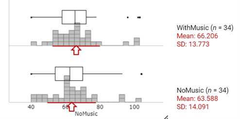
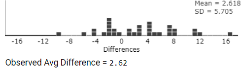
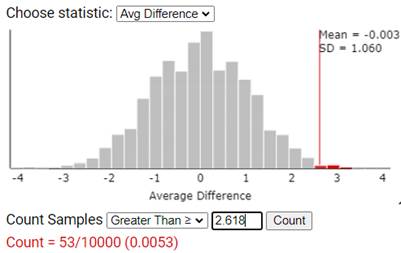
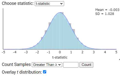
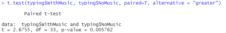
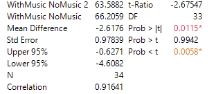
For each participant, we could randomly determine which of their typing speed measurements was measured with music and which without music. To do this, we would flip a coin. If the coin lands heads up, change the sign of the difference (so switch the music and no-music results). If the coin lands tails up, keep the results with their original labels (the difference would not change). Flip the coin for all 34 participants, find the (new) difference for each person and find the mean of these differences, \(\bar{x}_d\text{.}\) Repeat this "swapping" process a large number of times and look at the distribution of the \(\bar{x}_d\) values. Then count how many of these simulated \(\bar{x}_d\) values are at least as extreme as the \(-2.62\) we observed in our study (where "as extreme" would mean \(\bar{x} > 2.62\) and \(\bar{x} \lt -2.62\) for our two-sided alternative).

🔗

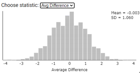
Pseudo code:

🔗

for i:1 to 1000
  for j: 1 to n
    multiplier = flip a coin (-1,1) w/ prob 0.5
    newdifference[j] = multiplier*olddiff[j]
  end loop
  calculate meandiff[i]=mean(newdifference)
end loop
pvalue=2*sum(meandiff[i] > 2.62) /1000

🔗

Copy and paste the original raw data (TypingMusic.txt) into the Matched Pairs applet (or type TypingMusic.txt into the data window and press Use Data twice):

🔗

View the data window, with one column for the speeds with music and a second column for the speeds without music (each row is one person). You can also include an initial column of identifiers (e.g., student IDs or initials). The dotplots should then show both sets of data, connecting the paired observations, and their differences.

🔗

🔗

8. Examine the distributions.

How many "high outliers" (fastest typers) are there in each condition? Are they related to each other?

🔗

Solution.

There are three high outliers in each condition. They belong to the same three individuals.

🔗

Check the Randomize box and press Randomize. For each pair, the applet will virtually "flip a coin" and if the coin lands heads, the two observations for that person will change positions. The new dotplots and the new set of differences for these rearranged values will be displayed. The mean of these differences will appear in the bottom dotplot.
🔗

🔗
Uncheck Animate. Press Randomize four more times to get a sense of the variability in the mean difference from repetition to repetition. Change the number of repetitions from 1 to 995 (for a total of 1000) and press Randomize.
🔗

🔗

🔗

9. Tracking the randomized values.

What do you notice about the high outliers after each shuffle?

🔗

Solution.

Notice that the same three people are the high outliers, but the two responses may swap between the treatment groups.

🔗

Example output:

Distribution of 1000 simulated mean differences from re-randomizations

🔗

10. Interpret Randomization Distribution.

Explain what distribution is being displayed in the bottom (grey) dotplot (what order of subtraction did the applet use?).

🔗

Solution.

This is the distribution of 1000 simulated \(\bar{x}_d\) values from 1000 re-randomizations where \(\bar{x}_d\) is calculated by subtracting the with-music speed from the no-music speed.

🔗

11. Mean of Distribution.

Where is the mean of the distribution of the average differences? Why should you expect that?

🔗

Solution.

The center is 0. This is expected because the groups are equally likely to end up with the higher mean.

🔗

12. Assess Observed Value.

How surprising does our observed value for the mean difference appear to be, under the simulation’s assumption that presence/absence of up-tempo music does not affect typing speed?

🔗

Solution.

The average difference observed by the student researchers (2.618) falls in the upper right tail of the distribution. It does appear to be a bit unlikely to happen under the assumption that presence/absence of music does not affect typing speed.

🔗

Use the applet to determine the proportion of simulated Average Differences that are more extreme than what we observed.
🔗

🔗

13. p-value and Conclusion.

Report the empirical p-value. What conclusion will you come to based on this p-value? Can you draw a cause-and-effect conclusion? For what population?

🔗

Hint.

Be sure to consider the alternative hypothesis when deciding what to consider as "more extreme."

🔗

Solution.

Example results:

🔗

Because the applet used a different direction of subtraction, we want to find the proportion of simulated values that are 2.618 or larger. With an approximate p-value of 0.0053 \(\lt\) 0.05, we reject the null hypothesis and find statistically significant evidence in favor of the alternative hypothesis, that long-run average typing speed is larger with the up-tempo music. We can draw a cause-and-effect conclusion with this small p-value, because the student employed random assignment in the ordering of the conditions. We don’t have a lot of information about how the sample was selected, but it does not appear to be random sampling and we should be cautious in generalizing these results beyond the musicians and athletes at this university.

🔗

Mathematical Model.

🔗

14. Normal Distribution Model.

Does the randomization distribution appear that it would be reasonably well-modeled by a normal distribution?

🔗

Yes
Correct! The randomization distribution appears reasonably symmetric and bell-shaped.
No
Look at the shape of the randomization distribution in the applet.

🔗

15. t-Distribution Model.

If you change the Statistic from Avg Difference to t-statistic (and check the Overlay t distribution box), do the standardized statistics appear well-modeled by a t-distribution?

🔗

Yes
Correct! The t-distribution overlays the randomization distribution well.
No
Check the overlay of the t-distribution on the randomization distribution in the applet.

🔗

Definitions: Paired t-test.

A paired t-test standardizes the mean of the differences from a matched-pairs design.

🔗

\begin{equation*} t = \frac{\bar{x}_{diff} - 0}{s_{diff}/\sqrt{n_{diff}}} \end{equation*}

🔗

where \(\bar{x}_{diff}\) is the sample mean of differences and \(s_{diff}\) is the sample standard deviation of the differences. The standardized statistic above assumes the hypothesized difference is zero, but this can be changed.

🔗

Technical conditions: When the distribution of differences is normally distributed or the sample size is large (e.g., \(n > 30\) pairs of observations), this t-statistic is well modeled by a t-distribution with \(n - 1\) degrees of freedom.

🔗

A paired t-confidence interval for \(\mu_d\) has the form

\begin{equation*} \bar{x}_{diff} \pm t_{n-1}^* \times (s_{diff}/\sqrt{n_{diff}}) \end{equation*}

🔗

Note: These are a special case of the one-sample t-procedures that can be applied to a single sample of quantitative data (see Investigation 2.5). In this case, variable of interest is the difference in the quantitative response for each observational unit pair.

🔗

16. Calculate and Interpret t-statistic.

Use the summary statistics to calculate, by hand, and then interpret the value of this standardized statistic.

🔗

Solution.

\(t = \frac{2.618 - 0}{5.71/\sqrt{34}} \approx 2.67\)

🔗

Interpretation: Our \(\bar{x}_d\) is 2.67 standard errors above the hypothesized \(\mu_d\) of 0.

🔗

17. Compare p-values.

Using the Overlay t distribution in the applet, how does the p-value compare to the empirical p-value from the simulated paired-randomization test? Do the t-procedures appear to be valid for these data?

🔗

Solution.

The standardized statistic is 2.68 and the p-value is 0.006. This is very similar to the p-value from the randomization test (0.005).

🔗

🔗

18. Confidence Interval.

Use the check box to display the 95% CI for average difference. Report and interpret this interval in context. Is the confidence interval consistent with the p-value? What additional information is provided by the confidence interval?

🔗

Solution.

95% CI: (0.66, 4.57), The long-run average difference in typing speeds (no music-music) is estimated to fall between 0.66 and 4.57 wpm with 95% confidence. We would have enough evidence to conclude that there is an effect of music, as this interval does not include zero. This is consistent with a p-value of 0.006. The additional information provided by the confidence interval is a plausible range for the mean difference in typing speed.

🔗

19. Verify with Software.

Verify your results using software.

🔗

Hint 1. R

In R: you can use the t.test command as before but specify the data are paired, e.g.,

🔗

> t.test(WithMusic, NoMusic, alternative="greater", conf.level = .95, paired=TRUE)

OR with stacked data

🔗

> t.test(speed~condition, alt="greater", paired=TRUE)

🔗

Hint 2. JMP

In JMP:

🔗

Choose Analyze > Specialized Modeling > Matched Pairs
🔗

🔗
Specify the two columns in the Y, Paired Response box and press OK.
🔗

🔗

The output will include the standardized statistic (t-Ratio), p-values, and confidence interval endpoints.

🔗

Solution.

R output:

🔗

JMP output:

🔗

Discussion.

To compare two groups on a quantitative variable, a more powerful study design than randomly assigning individuals to two groups, if possible, is to pair individuals (or take two measurements on each individual) and measure both responses in each pair (See Example 4.4). This pairing accounts for the variability from individual to individual and allows for a more direct comparison between the two conditions of interest. For example, if two measurements are taken on each individual, there should not be any other systematic differences between the measurements other than the treatment effect. Randomizing will still be important in determining the order of the two treatments, thereby eliminating order as a potential confounding variable. By accounting for the variability in individuals, this should increase the power of the test of significance, making it easier to detect a difference between the two conditions if one really exists. To analyze such data, perform a matched-pairs randomization test or a (one sample) t-test on the differences.

🔗

Note: The standard error of the difference in means is equivalent to \(SE(\bar{X}_1 - \bar{X}_2) = \sqrt{\frac{s_1^2 + s_2^2 - 2rs_1s_2}{n}}\text{,}\) which shows how the positive correlation between the two sets of measurements (\(r\)) reduces the estimated standard error of the statistic.

🔗

Study Conclusions.

A paired experiment comparing typing speeds with and without up-tempo classical music (Overture to Candide performed by the London Symphony Orchestra) found participants were significantly faster on average with the music. A paired t-test on the mean difference give a one-sided p-value of 0.006, similar to the simulation-based p-value using "random swapping" of the speeds to represent no difference between the two treatment conditions. We are 95% confident that participants like those in this study (e.g., college students, music students or athletes willing to help out a friend) type, on average, 0.63 to 4.61 more words per minute when listening to the up-tempo music. This evidence is much stronger than when we only compared the participants on their first tests, because of both effectively doubling the sample size and also reducing the amount of "unexplained variation" in the response variable. The person-to-person variation in typing speeds was around 15 wpm, compared to the person-to-person variation in difference in typing speeds which was around 5 wpm. A further analysis could compare the average improvement with music between the music students and the athletes.

🔗

Subsection 21.2.2 Practice Problem 4.9A

Checkpoint 21.2.1. Power with SD = 15.

Use statistical software to determine the power of detecting a difference of 5 wpm in a two-sample t-test if the sample standard deviations are 15 wpm. (You can assume a 5% level of significance and a one-sided alternative, as well as a total sample size of 34.)

🔗

Checkpoint 21.2.2. Power with SD = 5.

Repeat the previous question assuming the sample standard deviations are 5 wpm.

🔗

Checkpoint 21.2.3. Power for Paired t-test.

Use statistical software to determine the power of detecting a difference of 5 wpm in a one-sample paired t-test assuming the sample standard deviation of the differences is 5 wpm.

🔗

Checkpoint 21.2.4. Compare Power.

How does the power of the paired t-test compare to the power of the two-sample t-test? (Cite appropriate evidence.)

🔗

Subsection 21.2.3 Practice Problem 4.9B

Scientists have long been interested in whether there are physiological indicators of diseases such as schizophrenia. In a 1990 study by Suddath et. al., reported in Ramsey and Schafer (2002), researchers used magnetic resonance imaging to measure the volumes of various regions of the brain for a sample of 15 monozygotic twins, where one twin was affected by schizophrenia and other not ("unaffected"). The twins were found in a search through the United States and Canada, the ages ranged from 25 to 44 years, with 8 male and 7 female pairs. The data (in cubic centimeters) for the left hippocampus region of the brain are in hippocampus.txt. The primary research question is whether the data provide evidence of a difference in hippocampus volumes between those affected by schizophrenia and those unaffected.

🔗

Checkpoint 21.2.5. Calculate Differences.

Calculate the difference in hippocampus volumes for each pair of twins (unaffected \(-\) affected).

🔗

Checkpoint 21.2.6. Confidence Interval and Validity.

Calculate and interpret a 95% confidence interval for the mean volume difference using the paired t-interval. Also comment on the validity of this procedure.

🔗

Checkpoint 21.2.7. Statistical Significance.

Based on this confidence interval, is there statistically significant evidence that the mean difference in left hippocampus volumes is different from zero? Explain.

🔗

You have attempted of activities on this page.

🔗

Prev Top Next