Address the questions posed in the introduction about designing a comparison shopping study with adequate power.
Solution.
The original study had access to an inventory list and was able to use a systematic sample to select one item from each of 30 pages. This required the students to find each item in the store, but each student was only given one item to find. If you needed to find all the items yourself, you might consider a multistage sampling plan where you number the aisles, randomly select an aisle, then within the aisle you could randomly select a side, and then randomly select a shelf, and then randomly select a distance down the aisle. This randomly selects and finds the items all in one step! You could then find those same items at the second store (matched pairs) or repeat this process at the second store (independent samples).
In order to carry out our power calculations, we need to a make a few more assumptions. We were already told that we want to use a two-sided alternative with \(\alpha = 0.05\text{.}\) If we are doing a two-sample design, the distribution of differences in sample means will be approximately normal if the sample sizes are large enough (especially because we expect these price distributions to be skewed to the right), with standard deviation \(\sqrt{\frac{\sigma_1^2}{n_1} + \frac{\sigma_2^2}{n_2}}\text{.}\) So step one is to determine \(\sigma_1\) and \(\sigma_2\text{,}\) but of course we can’t know their values exactly, but we really just need ballpark values for now. In the earlier study, we had sample standard deviations of $1.66 and $1.74. We will be a bit conservative and will assume $2.00 for both stores.
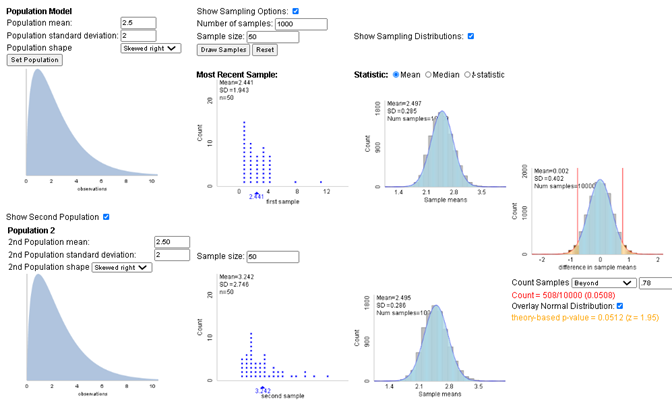
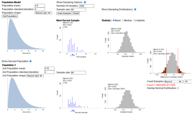
For illustration, let’s assume \(\mu_1 = \mu_2 = \$2.50\text{,}\) with \(\sigma_1 = \sigma_2 = 2\text{,}\) and \(n_1 = n_2 = 30\text{,}\) with population distributions that are skewed to the right. The simulation model (below, Two Populations applet) tells us that we would want to see about an $0.79 difference in the sample means to be convinced to reject the null hypothesis. This is our rejection region. And then if the second population mean is \(\mu_2 = \$2.70\text{,}\) we will find a difference in sample means at least as extreme as $0.80 in about 14% of samples, well below the desired 80%!
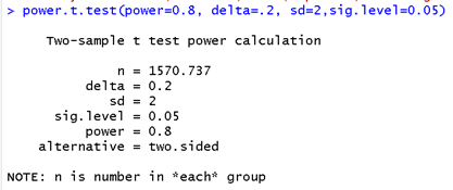
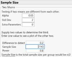
One solution is to this embarrassingly lower power is to increase the sample size. Turning to software, JMP and R report a necessary sample size of 1,571 products at each store.
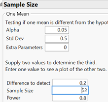
Another alternative is a paired design and a one-sample t-test. Suppose we assume \(\mu_d = 0\text{,}\) \(\sigma_d = 0.50\) (note, we are assuming a much smaller standard deviation in the differences than in the product prices, similar to what was observed in Investigation 4.10, the main advantage of the matched pairs design), and want to detect a mean price difference of $0.20 with 80% power. Software tells us, we need just 52 products.
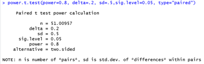
There is a huge improvement with the paired design, though our probability of detecting a difference is still only 80% when the average difference is actually 20 cents. This probability drops to about 53% with 28 items, so it’s important to aim for more observations than your power calculation reveals to account for attrition in the sample. But keep in mind that for a very small difference, especially with lots of natural variation in the responses, a very large sample size would be needed and may not be practical. It’s important to discuss "what is a meaningful difference to detect" with the subject matter experts.
