Investigation 3.10: Sleepy Drivers

Section 12.8 Investigation 3.10: Sleepy Drivers

Connor et al. (British Medical Journal, May 2002) reported on a study that investigated whether sleeplessness is related to car crashes. The researchers identified all drivers or passengers of eligible light vehicles who were admitted to a hospital or died as a result of a car crash on public roads in the Auckland, New Zealand region between April 1998 and July 1999.

🔗

Introduction image for Investigation 3.10

Through cluster sampling, they identified a sample of 571 drivers who had been involved in a crash resulting in injury and a sample of 588 drivers who had not been involved in such a crash as representative of people driving on the region’s roads during the study period. The researchers asked the individuals (or proxy interviewees) whether they had a full night’s sleep (at least seven hours mostly between 11pm and 7am) any night during the previous week. The researchers found that 61 of the 535 crash drivers who responded and 44 of the 588 "no crash" drivers had not gotten at least one full night’s sleep in the previous week.

🔗

Checkpoint 12.8.1. Identify Study Components.

Identify the observational units and variables in this study. Which variable would you consider the explanatory variable and which the response variable? Was this an observational study or an experiment? If observational, would it be considered a case-control, cohort, or cross-classified design?

🔗

Observational units:

🔗

Explanatory variable:

🔗

Response variable:

🔗

Type of study:

🔗

Solution.

Observational units: Drivers in Auckland, New Zealand

🔗

Explanatory variable: Whether got a full night’s sleep in previous week (categorical: yes/no)

🔗

Response variable: Whether involved in a car crash (categorical: yes/no)

🔗

Type of study: This is a case-control observational study. The researchers selected drivers who had crashes (cases) and drivers who had not (controls), then looked back at their sleep patterns.

🔗

Checkpoint 12.8.2. Create Two-Way Table.

Organize these sample data into a 2 × 2 table:

🔗

Table 12.8.3.

🔗

	No full night’s sleep in past week ("sleep deprived")	At least one full night’s sleep in past week ("not sleep deprived")	Sample sizes
Crash			535
No crash			588
Total			1123

Solution.

Table 12.8.4.

🔗

	No full night’s sleep	At least one full night’s sleep	Sample sizes
Crash	61	474	535
No crash	44	544	588
Total	105	1018	1123

🔗

Checkpoint 12.8.5. Calculate Appropriate Statistic.

Which statistic (odds ratio or relative risk) is most appropriate to calculate from this table, considering how the data were collected? Calculate and interpret this statistic. Does the value of this statistic support the researchers’ conjecture? Explain.

🔗

Solution.

Because this is a case-control study, the odds ratio is the most appropriate statistic. The researchers controlled the number of crash and no-crash drivers, so we cannot meaningfully calculate the risk of having a crash.

🔗

Odds ratio = (61/44) / (474/544) = 1.386 / 0.871 = 1.59

🔗

The odds of being in a crash if didn’t get a full night’s sleep were 1.59 times higher than the odds of being in a crash if did get at least one full night’s sleep. (Note: this is the same as the odds of not getting a full night’s sleep for the crash victims vs. the odds of not getting a full night’s sleep for the non-crash subjects.)

🔗

This does support the conjecture that sleeplessness is related to car crashes, as the odds ratio is notably greater than 1.

🔗

Statistical Inference.

🔗

Checkpoint 12.8.6. Simulation Design.

Outline the steps of a simulation that models the randomness in this study and helps you assess how unusual the statistic is that you calculated in checkpoint 5 when the null hypothesis is true. Include a statement of the null and alternative hypotheses for your choice of parameter.

🔗

Solution.

We could replicate the sampling design by sampling independently from two binomial processes with the same probability of success (this will model H₀: τ = 1). One process will represent the sampling of the crash victims (n = 535) and the other will represent the sampling of the no-crash population (n = 588).

🔗

Let \(\tau\) represent the population odds ratio.

🔗

H0: \(\tau\) = 1 (the odds of being sleep deprived are the same for crash and no-crash drivers)

🔗

Ha: \(\tau\) > 1 (the odds of being sleep deprived are higher for crash drivers)

🔗

Simulation steps:

🔗

Assume the null hypothesis is true, so use 105/1123 ≈ 0.0935 as the common probability of success (no full night’s sleep)

🔗
For the crash group, simulate 535 binomial observations with success probability 0.0935

🔗
For the no-crash group, simulate 588 binomial observations with success probability 0.0935

🔗
Calculate the odds ratio for this simulated sample

🔗
Repeat steps 2-4 many times (e.g., 10,000 times)

🔗
Find the proportion of simulated odds ratios that are at least as large as the observed value of 1.59

🔗

🔗

Aside

Checkpoint 12.8.7. Carry Out Simulation.

Use technology to carry out your simulation and draw your conclusions.

🔗

Hint.

Be careful of rounding issues in finding your p-value, make sure you are including observations as extreme as the observed in your count.

🔗

Solution.

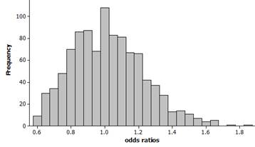
The distribution should appear skewed to the right with mean close to 1 and standard deviation around 0.21.

🔗

Example simulation results: mean ≈ 1.108, standard deviation ≈ 0.213

🔗

Simulation results showing the distribution of odds ratios under the null hypothesis

The observed ratio of 1.59 is a fair bit out in the tail of the distribution. Counting how many simulated odds ratios are 1.59 or larger, we find approximately 1% to 1.5% of the simulated values are at least this extreme.

🔗

Using Fisher’s Exact Test, the one-sided p-value is 0.0158.

🔗

This small p-value (approximately 0.016) provides strong evidence against the null hypothesis, suggesting that there is a relationship between sleep deprivation and car crashes in the population.

🔗

Checkpoint 12.8.8. Confidence Interval.

Calculate and interpret a 95% confidence interval for your choice of parameter.

🔗

Solution 1.

Theoretical standard error for the log odds ratio:

🔗

SE(ln odds ratio) = \(\sqrt{\frac{1}{61} + \frac{1}{44} + \frac{1}{474} + \frac{1}{544}}\) ≈ \(\sqrt{0.0164 + 0.0227 + 0.0021 + 0.0018}\) ≈ \(\sqrt{0.043}\) ≈ 0.2075

🔗

ln(1.59) ≈ 0.4637

🔗

95% CI for ln(odds ratio): 0.4637 ± 1.96(0.2075) = 0.4637 ± 0.4067 ≈ (0.057, 0.870)

🔗

Back-transform: exp(0.057, 0.870) ≈ (1.06, 2.39)

🔗

We are 95% confident that the odds of being in a car crash are 1.06 to 2.39 times larger for those without a full night’s sleep in the previous week compared to those with at least one full night’s sleep.

🔗

This interval does not capture one, so we have statistically significant evidence of an increase in odds for those without a full night’s sleep.

🔗

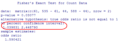
Solution 2. Solution using R

R output showing confidence interval calculation for odds ratio

🔗

Solution 3. Solution using JMP

JMP output showing confidence interval calculation for odds ratio

🔗

Checkpoint 12.8.9. Overall Conclusions.

Summarize (with justification) the conclusions you would draw from this study (using both the p-value and a confidence interval, and addressing both the population you are willing to generalize to and whether or not you are drawing a cause-and-effect conclusion).

🔗

Solution.

We have strong evidence (p-value = 0.0158) that sleep-deprived drivers have higher odds (6% to 139% higher) of being in a car crash, at least for drivers like these New Zealand drivers.

🔗

The 95% confidence interval (1.06, 2.39) indicates that the odds are approximately 1 to 2.4 times higher for sleepy drivers. Since this interval does not contain 1, we have statistically significant evidence of an association.

🔗

However, we cannot draw a cause-and-effect conclusion because this was an observational study. There could be confounding variables (e.g., driver experience, time of day, road conditions, alcohol use).

🔗

We should apply these results only to drivers in Auckland, New Zealand at that time, as that is the population from which the sample was drawn.

🔗

Study Conclusions.

The proportions of drivers who had not gotten a full night’s sleep in the previous week were 0.107 for the case group of drivers who had been involved in a crash, compared to 0.075 for the control group who had not. Because these proportions are small, and because of the awkward roles of the explanatory and response variables in this study (we would much rather make a statement about the proportion of sleepless drivers who are involved in crashes), the odds ratio is a more meaningful statistic to calculate. The sample odds of having missed out on a full night’s sleep were 1.59 times higher for the case group than for the control group. By the invariance of the odds ratio, we can also state that the sample odds of having an accident are 1.59 times (almost 60%) higher for those who do not get a full night sleep than those who do. The empirical p-value (less than 5%) provides moderately strong evidence that such an extreme value for the sample odds ratio is unlikely to have arisen by chance alone if the proportion of drivers with sleepless nights was 0.09 for both the population of "cases" and the population of "controls." (Using a one-sided Fisher’s Exact Test, we get p-value = 0.016.) A 95% confidence interval for the population odds ratio extends from 1.06 to 2.39 (1.04 to 2.45 with R). This interval provides statistically significant evidence that the population odds ratio exceeds 1.0 and that, with 95% confidence, the odds of having an accident are about 1 to 2.5 times higher for the sleepy drivers than for well rested drivers. We cannot attribute this association to a cause-and-effect relationship because this was an observational (case-control) study. We might also want to restrict our conclusions to New Zealand drivers.

🔗

Subsection 12.8.1 Practice Problem 3.10

Another landmark study on smoking began in 1952 (Hammond and Horn, 1958, "Smoking and death rates—Report on forty-four months of follow-up of 187,783 men: II. Death rates by cause," JAMA). They used 22,000 American Cancer Society volunteers as interviewers. Each interviewer was to ask 10 healthy white men between the ages of 50 and 69 to complete a questionnaire on smoking habits. Each year during the 44-month follow-up, the interviewer reported whether or not the man had died, and if so, how. They ended up tracking 187,783 men in nine states (CA, IL, IA, MI, MN, NJ, NY, PA, WI). Almost 188,000 were followed up by the volunteers through October 1955, during which time about 11,870 of the men had died, 488 from lung cancer. The following table classifies the men as having a history of regular cigarette smoking or not and whether or not they died from lung cancer. In this study, nonsmokers are grouped with occasional smokers, including pipe- and cigar-only smokers.

🔗

Table 12.8.10. Hammond and Horn Study

🔗