Example 4.1: Age Discrimination?

Section 22.1 Example 4.1: Age Discrimination?

Try these questions yourself before you use the solutions following to check your answers.

In Investigation 4.1 you considered the case of Robert Martin and whether the sample of 10 employees in his department provided evidence of age discrimination. Suppose we decide to focus on the long-run difference in mean ages for those laid-off and those retained for the decision making process used by this company.

🔗

Checkpoint 22.1.1. State Hypotheses.

State the null and alternative hypotheses, in symbols, for this study.

🔗

Hint.

Define your symbols.

🔗

Solution.

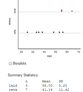
Let \(\mu_{fired} - \mu_{not fired}\) represent the difference in the average age of people that would be laid-off, in the long run (by the overall process), and the average age of the people who would be retained. (Don’t worry too much at this point about which stage of the firing process this analysis considers. Just keep in mind that we are trying to say something beyond the observed means. We believe there is some underlying difference in means and these data provide an estimate.)

🔗

\begin{gather*} H_0: \mu_{fired} - \mu_{not fired} = 0 \text{ (no overall difference in the average ages of those getting fired and not)}\\ H_a: \mu_{fired} - \mu_{not fired} > 0 \text{ (those getting fired will tend to have higher ages than those not)} \end{gather*}

🔗

Checkpoint 22.1.2. Observed Statistic.

Recall the observed value of the sample statistic (in years).

🔗

Solution.

\(\bar{x}_1 - \bar{x}_2 = 58.00 - 41.14 = 16.86\) years

🔗

Checkpoint 22.1.3. Randomization Test.

Simulate a randomization test for these data and state your conclusion at the 0.01 level of significance.

🔗

Aside: Comparing Groups Applet.

Solution.

Using the Comparing Groups (Quantitative) applet, the empirical p-value (remembering to match the direction of subtraction, which may vary depending on how you pasted the data in), the output below shows an empirical p-value of 0.0225. Because 0.0225 > 0.01, we would not reject the null hypothesis at the 0.01 level and conclude that this firing process was not more likely to fire individuals with larger ages.

🔗

Randomization distribution showing empirical p-value of 0.0225

Note: You could also carry out this simulation using software, e.g., in R:

🔗

I = 10000; diff = 0			
for (i in 1:I){						
  rerandom = sample(age)
  diff[i] = mean(rerandom[1:3])-mean(rerandom[4:10])
}

🔗

Checkpoint 22.1.4. Two-Sample t-Test.

Carry out a two-sample t-test for these data and hypotheses, and state your conclusion at the 0.01 level of significance.

🔗

Aside: Theory-Based Inference Applet.

Solution.

A two-sample t-test using software:

🔗

JMP

🔗

Now p-value \(\lt\) 0.01, and we would reject the null hypothesis at the 0.01 level and conclude that this firing process was more likely to fire individuals with larger ages.

🔗

Checkpoint 22.1.5. Compare Analyses.

Do these analyses reach the same conclusion? If not, which analysis should be used? Explain.

🔗

Solution.

The two-sample t-test yields a much smaller p-value, about 0.006, which implies much stronger evidence of an underlying age difference between the two populations (fired and not fired). However, because of the small sample sizes (especially with the unbalanced groups), we would have major concerns about using the t-procedures for this study. The empirical p-value from the simulated randomization test is more trustworthy. In fact, in this study, it’s probably more work than we need to do, because with only 120 possible combinations it is not unreasonable to calculate the exact p-value.

🔗

You have attempted of activities on this page.

🔗

Prev Top Next