
Section 12.7 Summary of Inference for Odds Ratio

For tables of the form:
\(A\) \(B\)
\(C\) \(D\)
\(A + C\) \(B + D\)

Odds Ratio Procedures.

Statistic: Odds ratio (typically set up to be larger than one) = \(\frac{A \times D}{B \times C}\) or equivalently \(\frac{\text{odds}_1}{\text{odds}_2} = \frac{\frac{\hat{p}_1}{1-\hat{p}_1}}{\frac{\hat{p}_2}{1-\hat{p}_2}}\)
Hypotheses: \(H_0: \tau = 1\) or \(\ln(\tau) = 0\text{;}\) \(H_a: \tau < 1\text{,}\) \(\tau > 1\text{,}\) or \(\tau \neq 1\) (or equivalently using \(\ln(\tau)\))
p-value: Fisher’s Exact Test or normal approximation on \(\ln(\text{odds ratio})\)
Confidence interval for \(\tau\text{:}\) Exponentiate endpoints of
\begin{equation*} \ln\left(\frac{A \times D}{B \times C}\right) \pm z^*\sqrt{\frac{1}{A}+\frac{1}{B}+\frac{1}{C}+\frac{1}{D}} \end{equation*}
Technology:
  • In Two-way Tables applet: Choose Odds Ratio as statistic and check box for 95% CI
  • In R: You can install the fmsb package and use the oddsratio command.
    fmsb::oddsratio(A, B, C, D, conf.level, p.calc.by.independence = TRUE)
  • In JMP: From the Contingency Analysis hot spot, choose Odds Ratio

Technology Detour – Simulating Random Assignment (two-way tables).

  1. Simulate a random sample (number of successes for group 1) using the hypergeometric distribution
  2. Calculate the number of successes for group 2 (total successes – number of successes group 1)
  3. Convert the counts to proportions
  4. Calculate the odds for each group and the odds ratio
  5. Calculate the log-odds ratio
Keep in mind you can use "log" to calculate the natural logs of values. Also recall how you created a Boolean expression in Investigation 3.1 to find the p-value from the simulated results.
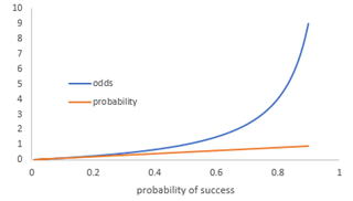
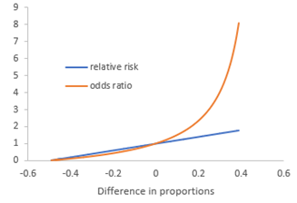
The graphs below show how (a) the probability of success and odds of success are related and (b) how relative risk and odds ratios are similar when the difference in proportions is small. Also note that when the difference in proportions is zero, the relative risk and the odds ratio are both one.
The table below demonstrates the invariance property of the odds ratio for Investigation 3.9. Notice that the odds ratio remains constant at 9.385 regardless of how we set up the comparison, while the relative risk changes depending on the setup.
Odds Ratio Relative Risk
Of lung cancer comparing smokers to non-smokers \(\frac{583/576}{22/204} = 9.385\) \(\frac{583/1159}{22/226} = 5.17\)
Of not having lung cancer comparing non-smokers to smokers \(\frac{204/22}{576/583} = 9.385\) \(\frac{204/226}{576/1159} = 1.816\)
Of not having lung cancer comparing smokers to non-smokers \(\frac{576/583}{204/22} = 0.1065\) \(\frac{576/1159}{204/226} = 0.551\)
Of lung cancer comparing non-smokers to smokers \(\frac{22/204}{583/576} = 0.1065\) \(\frac{22/226}{583/1159} = 0.194\)
Of being a smoker comparing lung cancer patients to controls \(\frac{583/22}{576/204} = 9.385\) \(\frac{583/605}{576/780} = 1.305\)
You have attempted of activities on this page.