Section20.1Investigation 4.4: Lingering Effects of Sleep Deprivation
The previous section focused on quantitative data arising from two independent random samples. This section will focus on quantitative data arising from randomized experiments. We will again consider simulation-based, exact, and theory-based p-values, as well as what assumptions we need to make for confidence intervals.
Researchers have established that sleep deprivation has a harmful effect on visual learning (the subject does not consolidate information to improve on the task). Stickgold, James, and Hobson (2000) investigated whether subjects could “make up” for sleep deprivation by getting a full night’s sleep in subsequent nights.
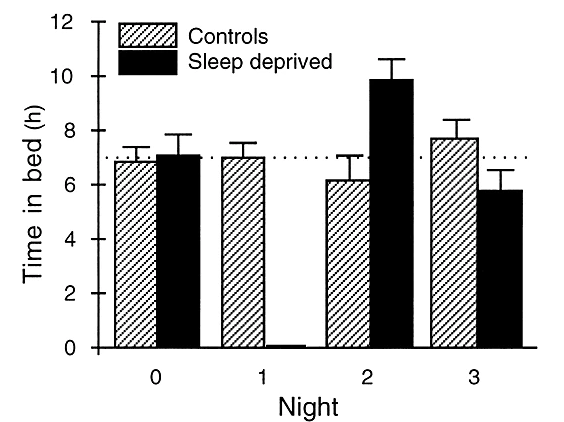
This study involved randomly assigning 21 subjects (volunteers between the ages of 18 and 25) to one of two groups: one group was deprived of sleep on the night following training with a visual discrimination task, and the other group was permitted unrestricted sleep on that first night. Both groups were allowed unrestricted sleep on the following two nights, and then were re-tested on the third day.
Subjects’ performance on the test was recorded as the minimum time (in milliseconds) between stimuli appearing on a computer screen for which they could accurately report what they had seen on the screen. Previous studies had shown that subjects deprived of sleep performed significantly worse the following day, but it was not clear how long these negative effects would last. The data presented here are the improvements in reaction times (in milliseconds), so a negative value indicates a decrease in performance.
Is your alternative hypothesis one-sided or two-sided? What does this imply about the types of response values you would expect to see in each treatment group?
The alternative hypothesis is one-sided; we expect to see positive improvement scores in each group, but higher scores in the unrestricted sleep group.
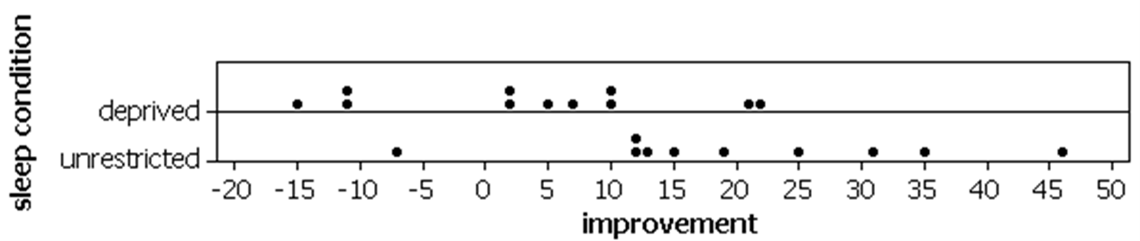
Are all the improvement scores in one group higher than all the improvement scores in the other group? Is there a tendency for higher improvement scores in one group three days later?
On average, the improvement score was higher for unrestricted group. We see a tendency for higher improvement scores in the unrestricted group (the dotplot is shifted to the right compared to the sleep deprived group dotplot).
There are several ways we could choose to measure the tendency observed in Question 5. A common choice of statistic is of course the difference in group means. Calculate this statistic by subtracting the “deprived” group’s value from the “unrestricted” group’s value.
Is it possible that the differences seen here could have occurred just by chance variation, due to the random assignment of subjects to groups, even if there were really no effect of the sleep condition on improvement?
As usual, we want to know how plausible it is for us to obtain a difference in sample means at least as extreme as the observed value by chance alone. What is the source of “chance” in this study?
Outline the steps of a simulation analysis that would explore the “could have been” outcomes under the null hypothesis by modelling the randomness described in Question 8.
We want to simulate the random assignment by assuming everyone would get the same improvement score, regardless of which group they end up in, and randomly assign the subjects into 2 groups of \(n_1 = 11\) and \(n_2 = 10\text{.}\) Then see how frequently you get \(\bar{x}_1 - \bar{x}_2 > 15.92\text{.}\)
As with the “dolphin therapy” experiment from Chapter 3, we again need to judge the strength of evidence that the experimental data provide in support of the researchers’ conjecture that sleep deprivation has a harmful effect on learning. We are now working with a quantitative response variable rather than a categorical one, but we will use the same basic logic of statistical significance: We will ask whether the observed experimental results are very unlikely to have occurred by chance variation if the explanatory variable has no effect, that is, if the values in the two groups are interchangeable. To simulate this randomization test: We will take the observed response variable outcomes, randomly distribute these numerical values between the two groups, compute the statistic of interest (e.g., the difference in group means), repeat this process a large number of times, and see how often the random assignment process alone produces a difference in group means as extreme as in the actual research study. This is similar to what you considered in Investigation 4.1. However, this time it is not really feasible to list out all possible \(C(21,10) = 352,716\) random assignments and consider the value of the statistic for each one, so we will simulate a large number of random assignments instead. Note, we need to know the value of \((\bar{x}_1 - \bar{x}_2)\text{,}\) not just the “number of successes” as with the dolphin therapy study.
Take a set of 21 index cards, and write each of the improvement values on a card. Then shuffle the cards and deal out 10 of them to represent the subjects randomly assigned to the “unrestricted sleep” group and 11 to represent the “sleep deprived group.” Calculate the mean of the improvements in each group. Then calculate the difference in group means, subtracting in the same order as before.
Is your simulated result for the difference in means as extreme as the actual experimental result? Explain. Why is looking at this one simulated difference not enough to assess statistical significance?
Results will vary. Looking at just one simulated difference is not enough because we need to understand the entire distribution of what could happen by chance alone to determine how often (what proportion of the time) random assignment alone produces results as extreme as what we observed.
Simulating more repetitions would provide a better understanding of how significant (i.e., unlikely to have happened by random assignment alone) the observed experimental results are. In other words, more repetitions will enable us to approximate the p-value more accurately. We will again turn to technology to perform the simulation more quickly and efficiently.
Open the Comparing Groups (Quantitative) applet. You will see dotplots of the research results. Verify the calculation of the observed difference in group means. (This applet subtracts the top row from the bottom row.)
The applet combines all the scores into one pile, reassigns the group labels (red and black coloring) at random, and then redistributes the observations to the two treatment groups, just like you did with the index cards.
Press Shuffle Responses four more times. With each new “could have been” result (each new random assignment), the applet calculates the difference in group means and adds a dot to the dotplot to the right.
Each dot is the value of \(\bar{x}_1 - \bar{x}_2\) after one reshuffling of the data values (What is the difference in sample means with each random assignment?).
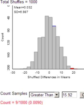
Now enter the observed difference in group means (Question 6) from the research study into the Count Samples box, use the Greater Than option (to match our alternative hypothesis), and press the Count button.
Provide an interpretation of this p-value in context (make sure you address the statistic, the source of the randomness in the study, and what you mean by “more extreme”).
The p-value is the percentage of random assignments, when the null hypothesis is true (\(H_0: \mu_{\text{unrestricted}} - \mu_{\text{deprived}} = 0\text{,}\) no treatment effect) that will have \(\bar{x}_{\text{unrestricted}} - \bar{x}_{\text{deprived}} \geq 15.92\) by chance (random sampling) alone.
What conclusion would you draw from this simulation analysis regarding the question of whether the learning improvements in the sleep deprived group are statistically significantly lower (on average) than those in the unrestricted sleep group? Also explain the reasoning process by which your conclusion follows from the simulation results.
With a p-value below 0.01, reject \(H_0\) because p-value is small, in favor of \(H_a: \mu_{\text{unrestricted}} - \mu_{\text{deprived}} > 0\text{.}\) We have convincing evidence that the observed difference in means is not just due to random chance but instead that the underlying treatment mean for the unrestricted group is higher than for the sleep deprived treatment.
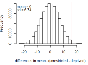
Although not as convenient as before, we can determine the exact p-value for this randomization test by considering all the different possible random assignments of these 21 subjects into groups of 11 and 10, determining the difference in means (or medians) for each, and then counting how many are at least as extreme as the observed difference.
The following histogram (produced using the combn function in R, from the combinat package, assuming imprvs contains the response variable values) shows the distribution of all 352,716 possible differences in group means.
indices = 1:21
allcombs = combn(21, 10)

diffs = 1:ncol(allcombs)

for (i in 1:ncol(allcombs)){
  group1=imprvs[allcombs[,i]]
  group2=imprvs[setdiff(indices, allcombs[,i])]
  diffs[i]=mean(group1)-mean(group2)
}

hist(diffs)
abline(v=15.92, col=2)

# approx. run time: 1 min
22.Compare Simulation to Exact.
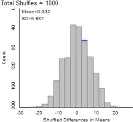
Do your simulation results reasonably approximate this null distribution?
It turns out that 2533 of the 352,716 different random assignments produce a difference in group means of 15.92 milliseconds or larger. Use this information to determine the exact p-value of this randomization test. Is the approximate p-value from your simulation close?
The exact randomization distribution consists of every possible random assignment and calculates the statistic of interest (e.g., difference in means) for each one. Then we simply count how many of the configurations result in a value of the statistic at least as extreme (as defined by the alternative hypothesis) as the actual observed result. As you might expect, it can be extremely tedious, even with computers, to list out all of these possible random assignments. And these group sizes are relatively small! One shortcut is to only count how many assignments give results more extreme than the one observed, but as you will see we can often appeal to a mathematical model as well.
Look at the distribution of the statistic, including the mean and standard deviation, and count how many of the simulated statistics are as or more extreme as the observed.
These data come from a randomized, comparative experiment. The dotplots and descriptive statistics reveal that, even three days later, the sleep-deprived subjects tended (on average) to have lower improvements than those permitted unrestricted sleep. To investigate whether this difference is larger than could be expected from random assignment alone (assuming no real difference between the two treatment conditions, our null hypothesis), you simulated a randomization test by assigning the 21 measurements (improvement scores) to the two groups at random. You should have found that random assignment alone rarely produced differences in group means as extreme as in the actual study (the “exact” p-value is less than 0.01). Thus, we have fairly strong evidence that the average learning improvement is genuinely lower for the sleep deprived subjects. Moreover, because this was a randomized comparative experiment and not an observational study, we can draw a causal conclusion that the sleep deprivation was the cause of the lower learning improvements. However, the subjects were college-aged volunteers, so we may not want to generalize these results to a much different population.
Explain how the simulation analysis conducted in this investigation differs from Investigation 4.2. (What is the random process being simulated? What assumptions are underlying the simulation?)
In Investigation 4.2 (comparing elephant walking distances), we simulated the random sampling process from two populations under the assumption that the population means are equal. In Investigation 4.4, we simulated the random assignment process in an experiment under the assumption that the treatment has no effect (so the response values would be the same regardless of which group the subject was assigned to). Investigation 4.2 deals with observational data and random sampling; Investigation 4.4 deals with experimental data and random assignment.
Produce numerical and graphical summaries for the data in FakeSleepDeprivation.txt, representing a new set of 21 responses for the sleep deprivation study. Comment on how the shapes, centers, and variability for the two distributions compare between these data and the original data.
Use technology (see Technology Detour) to carry out a randomization test to compare the improvements for the sleep deprived and unrestricted sleep groups using the hypothetical data. Indicate how you approximated the p-value.
How does the p-value for the hypothetical data compare to the p-value for the original data? Explain why this makes sense based on what you learned about how the data sets compared in part (a).