ISCAM: Investigating Statistical Concepts, Applications, and Methods

The observational units are the 50 states and the District of Columbia. The response variable of interest is the percentage change in traffic fatalities from 1995 to 1996 (quantitative). This is an observational study because the researchers did not randomly assign which states would increase their speed limits.

The following graphical display is dotplots of the percentage change in traffic fatalities for each state (and D.C.) in the two groups on the same scale:

Because the distributions are reasonably symmetric, it makes sense to report the means and standard deviations as the numerical summaries:

These results indicate that there is a tendency for the percentage change in traffic fatalities to be higher in those states that increase their speed limits. This tendency is also seen in stacked boxplots:

The boxplots also reveal an outlier, the District of Columbia, which did not change its speed limit and had an unusually high decrease in the percentage change of accidents.

These summaries also reveal that the two sample distributions are reasonably similar in shape and variability.

In considering the technical conditions, we see that the sample sizes (19 and 32) are reasonably large. Coupled with the normal shaped sample distributions, the normality/large sample size conditions appears to be satisfied for us to use the t-distribution.

Let \(\mu_{no} - \mu_{yes}\) represent the true "effect" of increasing the speed limit on the traffic fatality rate (states that didn’t change speed limit – states that did change speed limit)

\(H_0: \mu_{no} - \mu_{yes} = 0\)

(there is no true effect from increasing the speed limit)

\(H_a: \mu_{no} - \mu_{yes} \lt 0\)

(increasing the speed limit leads to an increase in traffic fatalities,higher average percentage change with increase in speed limit)

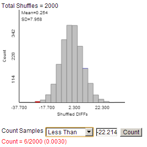
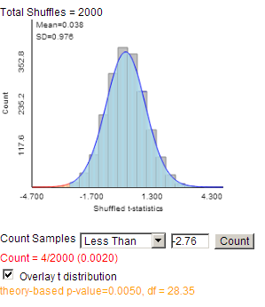
We can apply a randomization test that would look at what would happen if these groups were mixed up with no difference between the "no" group and the "yes" group.

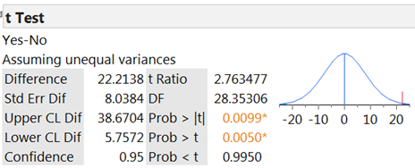
We can also approximate this randomization distribution with the two-sample t-procedure. In this case, the (unpooled) standardized statistic will be \(t = \frac{-8.53 - 13.69}{\sqrt{\frac{31^2}{19} + \frac{22^2}{32}}} = -2.74\)

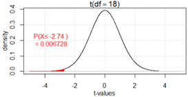
If we approximate the degrees of freedom by \(\min(19-1, 32-1) = 18\text{,}\) then we find the one-sided p-value to be:

> iscamtprob(-2.74, 18, "below")
probability: 0.006728

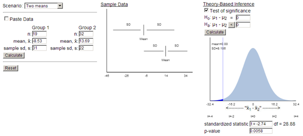
These calculations are confirmed with technology (with different df approximations):

Note: Our "by hand" method (using df = 18) is conservative in that the p-value found will be larger than the actual p-value as seen here.

Such a small p-value (0.005 \(\lt\) 0.01) reveals that we would observe such a large difference in group means by random assignment alone if there was no treatment effect only about 5 times in 1000, convincing us that the observed difference in the group means is larger than what we would expect just from random assignment. We have strong evidence that something other than "random chance" led to this difference. However, we cannot attribute the difference solely to the speed limit change because this was not actually a randomized experiment. As the states self-selected, there could be confounding variables that help to explain the larger increase in fatality rates in states that increased their speed limit.

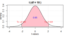
Because we rejected the null hypothesis, we are also interested in examining a confidence interval to estimate the size of the treatment effect. We first approximate the \(t^*\) critical value for say 95% confidence, again using \(\min(19-1, 32-1) = 18\) as the degrees of freedom.

> iscaminvt(.95, 18, "between")
There is 0.95 probability between -2.101 and 2.101

Then the 95% confidence interval can be calculated:

We are 95% confident that the true "treatment effect" is in this interval or that the mean percentage increase in traffic fatality rates is between 5.4 percentage points to 39.1 percentage points higher in states that increase their speed limit compared to states that do not increase their speed limit (continuing to be careful not to state this as a cause and effect relationship).

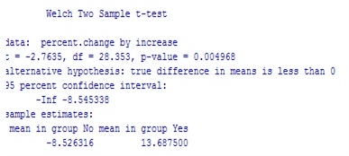
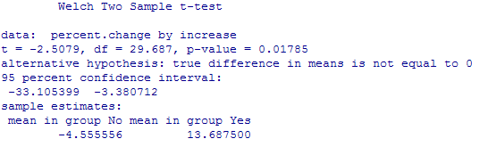
Before we complete this analysis, it is worthwhile to investigate the amount of influence that the outlier (the District of Columbia) has on the results, especially because D.C. does have different characteristics from the states in general. The updated R output (two-sided p-value) is below:

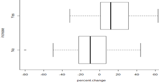
As we might have guessed, the mean increase in fatalities for the "No" group has increased so that the difference in the group means is less extreme. This leads to a less extreme standardized statistic and a larger p-value (one-sided p-value = 0.01785/2 = 0.0089) so somewhat weaker evidence against the null hypothesis in favor of the one-sided alternative hypothesis.

The other technical condition is that we have independent random samples or random assignment to groups. We do not have either in this study, because we are examining the population of all states (and D.C.), and the states self-selected whether they changed their speed limit. Thus, any p-value we calculate is in a sense hypothetical because we have all the states here, we might ask the question: would the two groups look this different if whether or not they increased their speed limit had been assigned at random?

So the above p-value measures how often we would see a difference in group means at least this large based on random assignment to the two groups if there were no true treatment effect. Although this p-value is hypothetical, we still have some sense that the difference observed between the groups is larger than we would expect to see "by chance" even in a situation like this where it is not feasible to carry out a true randomized experiment. This gives some information that can be used in policy decisions but we must be careful not to overstate the attribution to the speed limit change.