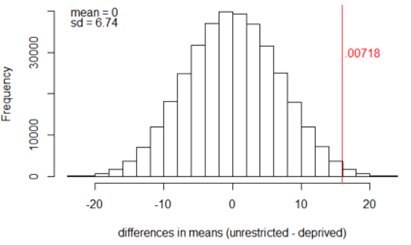
Reconsider the exact randomization distribution of the differences in sample means for the Sleep Deprivation study. Previously you determined simulation-based p-values and the exact p-value. Now we will explore modeling the randomization distribution of the difference in sample means with a probability distribution.
Suppose you want to use the normal model to approximate the p-value for obtaining a difference in means of 15.92 or larger under the null hypothesis or to compute a confidence interval. What other information do you need to know?
Compare this to the standard deviation you observed in the applet/for the exact randomization distribution. In particular, does this formula appear to over- or under-estimate the variability?
In Investigation 4.2, we stated that \(SD(\bar{X}_1-\bar{X}_2) = \sqrt{\frac{\sigma_1^2}{n_1} + \frac{\sigma_2^2}{n_2}}\text{,}\) because under the assumption that the two samples are independent, variances add. In a randomization test, however, the two samples are not independent: If one group gets all of the large responses, the other group must have all of the small responses and the difference in group means will be large. Consequently, the standard error formula from Investigation 4.2 will underestimate the shuffle-to-shuffle variation in the statistic. The discrepancy between the standard deviations for the difference in means is largest when the groups are more different: When we shuffle the responses back to the groups, any value can go into either group, but if there is a genuine difference between the treatments, then a score of 40 would be unlikely to come from say the deprived treatment. So how do we estimate the standard deviation of the randomization distribution? Turns out, we are less concerned with that. What we really want to be able to do is predict the behavior of the standardized statistic.
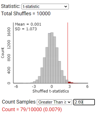
Use the Comparing Groups (Quantitative) applet to create a re-randomization null distribution. Change the Statistic pull-down menu to t-statistic and find the p-value using the value in Question 4. Is this the same p-value we found when we used the difference in means as the statistic in Investigation 4.4, Question 4?
If we use similar code to that in Investigation 4.4 to find the exact distribution of these t-statistics, we can find the exact p-value for the t-statistic is 0.00748. Is this similar to the simulation results?
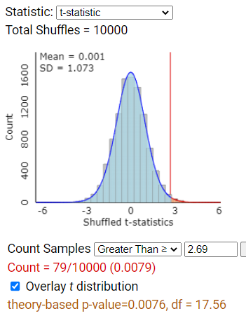
Correct! The t-distribution provides a reasonable model for the simulated null distribution, and its p-value reasonably approximates the exact p-value.
(a) Yes, (b) No
The t-distribution does provide a reasonable model, but the p-value from the t-distribution also reasonably approximates the exact p-value.
(a) No, (b) Yes
Actually, the t-distribution does provide a reasonable model for the simulated null distribution.
(a) No, (b) No
Actually, the t-distribution provides a reasonable model and its p-value reasonably approximates the exact p-value.
Solution.
The t distribution should provide a reasonable model.
The t-distribution comes to the rescue again, compensating for the underestimation in the variability, and in most situations (moderate and large sample sizes) gives an adequate approximation to the exact randomization distribution. Note the applet reports 17.56 as the degrees of freedom. This comes from the Welch-Satterthwaite approximation because the exact degrees of freedom are unknown in this case.
We will consider the t distribution to be a reasonable approximation for the randomization distribution of the t statistic as long as either (similar to what you witnessed in Investigation 4.2):
The data in both groups are symmetric and bell-shaped. When this is the case, we have evidence that the “treatment populations” are normally distributed. When this is true, the randomization distribution of the differences in group means will also follow a normal distribution.
The two sample sizes are large. Typically, the sample sizes can be as small as 5, especially if the two groups have similar sample sizes and similar distribution shapes, but conventionally 20 is used as cut-off for how large each sample should be to use this approximation. Examine graphs of your data first. If the sample distributions are not symmetric or have unusual observations, you will want larger sample sizes.
In summary, we will often apply the same two-sample t-procedures to both randomized experiments and to independent random samples. The distinction between these two sources of randomness will be most important in drawing your final conclusions (e.g., causation, generalizability). The advantage to the t-procedures over the exact randomization distribution is convenience, especially in calculating a confidence interval.
Write a one-sentence interpretation of this interval in context, being especially clear how you are defining the parameter for this randomized experiment.
We are 95% confident the long-run average improvement scores for those who are not sleep deprived are between 3.44 and 28.40 ms larger than for those who are sleep deprived.
The approximate p-value from the (unpooled, independent samples) two-sample t-test (0.0076, df = 17.56) also provides very strong evidence that the observed difference between the two groups did not arise by chance alone. Therefore, if we were to perform unlimited administrations of the same training and reaction time test under the exact same conditions, we have convincing evidence that the long-run mean of all improvement scores that an individual would have under sleep deprivation is lower, three days later, than the theoretical mean of all improvement scores that an individual would have with unrestricted sleep (i.e., \(\mu_{\text{sleepdeprived}} < \mu_{\text{unrestricted}}\)). We are 95% confident that the long-run mean improvement under the “no restriction” treatment is 3.44 to 28.40 ms faster that the long-run mean improvement under the “sleep deprivation” treatment. However, we still need to worry about what larger population these individuals represent.
Recall the study on children’s television viewing habits from Practice Problem 2.6B and Practice Problem 4.3B. One school incorporated a new curriculum, the other school did not.
The researchers want to decide whether the long-run mean number of hours of television viewing per week is lower after 6 months with the intervention than without the intervention. State the null and alternative hypotheses. If you use any symbols, make sure you clearly define them first.
Carry out a two-sample t-test. Include your output (indicating how found) and provide a one-sentence interpretation of the p-value in context (make sure you address the statistic, the source of the randomness in the study, and what you mean by “more extreme”).
The population distributions are likely skewed (bounded below by zero, SD similar to mean). Explain why the nonnormality of these distributions does not hinder the validity of using this t-test procedure.