Section13.3Investigation 3.2: Nightlights and Near-sightedness
Exercises13.3.1The Study
Myopia, or near-sightedness, typically develops during the childhood years. Several studies have explored whether there is an association between development of myopia and the use of night-lights with infants. Quinn, Shin, Maguire, and Stone (1999) examined the type of light children aged 2-16 were exposed to. The following two-way table classifies the children’s eye condition and whether or not they slept with some kind of light (e.g., a night light or full room light) or in darkness.
Between January and June 1998, the parents of 479 children who were seen as outpatients in a university pediatric ophthalmology clinic completed a questionnaire (children who had already developed serious eye conditions were excluded). One of the questions asked was "Under which lighting condition did/does your child sleep at night?" before the age of 2 years.
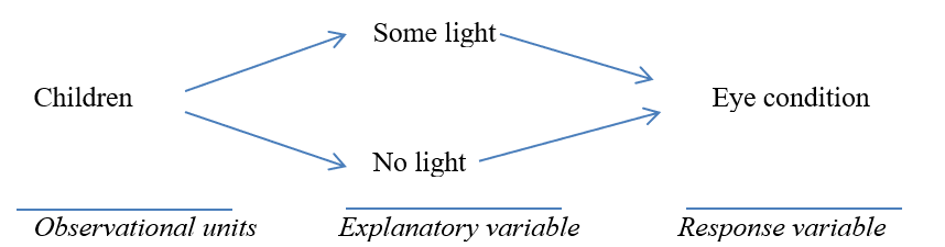
When we have two variables, we often specify one to be the explanatory variable and the other to be the response variable. The explanatory variable is the one that we think might be influencing or explaining changes in the response variable, the outcomes of interest.
Explanatory variable: Lighting condition; Response variable: Eye condition. The lighting condition came first in time (before age 2) and we are interested in whether it affects later eye condition.
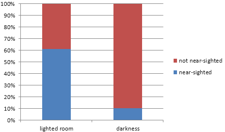
Calculate conditional proportions to measure the difference in the rate of near sightedness between the children with and without lighted rooms in this sample. (Use appropriate symbols.) Also produce a segmented bar graph to compare the eye condition of the two lighting groups.
Comment on what your numbers and graph reveals about differences in eye condition between these lighting groups. Do you think this difference will be statistically significant? Explain.
The segmented bar graph should show a much larger proportion of near-sighted children in the "some light" group compared to the "darkness" group. This difference appears very large and should be statistically significant.
In the previous investigation, the researchers literally took two distinct random samples from two different groups of teens. In this study, the data arose from one sample and each child in the sample was classified according to two variables: lighting condition and eye condition. A natural research question here might be "Does use of nightlights and room lights increase the rate of near-sightedness in children?" In such a situation, we can instead phrase our hypotheses in terms of the association between the two variables:
Since we have one sample classified by two variables rather than two separate samples, we could simulate by randomly assigning the 479 children to the two lighting conditions in the same proportions as observed (307 to "some light" and 172 to "darkness"), keeping the total number of near-sighted children fixed at 206. This would simulate the null hypothesis that lighting condition and eye condition are not associated.
It turns out, it will be valid to use the same inferential analysis procedures here as in Investigation 3.1 as long as the samples (e.g., room light, darkness) can be considered independent of each other. One counter example would be if the observational units had been paired in some way (e.g., brothers and sisters). But if we don’t believe the responses of particular children in lit rooms in this study in any way relate to the responses of particular children in the dark rooms, we consider the samples independent, even though they weren’t literally sampled separately. So we can use the same Central Limit Theorem to specify a normal distribution as a model of the sampling distribution of the difference in the two sample proportions.
Use technology to perform a two-sample \(z\)-test to compare the proportion with near sightedness between these two groups. Report the standardized statistic and p-value. Also report and interpret a 95% confidence interval from these data.
Interpretation: We are 95% confident that the probability of near-sightedness is between 0.44 and 0.58 higher for children who slept with some light compared to those who slept in darkness before age 2.
Because the p-value is so small, would you be willing to conclude that the use of lights causes an increase in the probability of near-sightedness in children? Explain. If not, suggest a possible alternative explanation for the significantly higher likelihood of near sightedness for children with lighting in their rooms.
No, we cannot conclude causation from this observational study. A possible confounding variable is the parents’ eye condition. Parents who are near-sighted may be more likely to use lighting in their children’s rooms (because they have trouble seeing in the dark), and children of near-sighted parents are more likely to be near-sighted themselves due to genetics. This provides an alternative explanation for the association without the lighting causing the near-sightedness.
When we find a highly significant difference between two groups, although we can conclude a significant association between the explanatory and response variables, we are not always willing to draw a cause-and-effect conclusion between the two variables. Though many wanted to use this study as evidence that it was the lighting that caused the higher rate of near-sightedness, for all we know it could have been that children with poorer vision asked for more light to be used in their rooms. Or there could even be a third variable that is related to the first two which could provide the real explanation for the observed association. Such a variable is called a confounding variable.
In some studies, we may consider one variable the explanatory variable that we suspect has an effect on the response variable. However, in some studies often there may be other confounding variables that also differ between the explanatory variable groups and have a potential effect on the response variable.
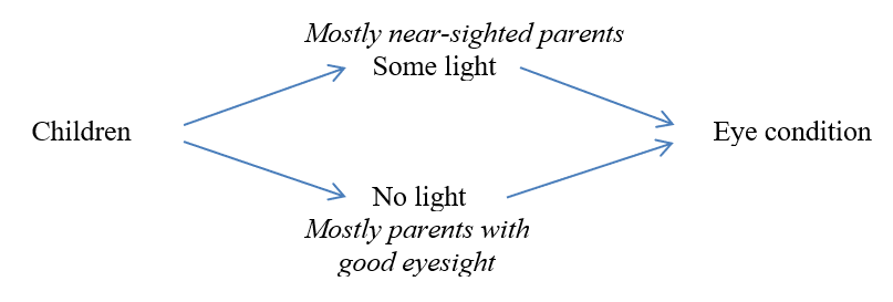
Your alternative explanation in Question 5 probably identified a potential confounding variable. For example, eye condition of the parents may be related to the explanatory variable (parents with poorer sight are more likely to use room lighting) and to the response variable (children of near-sighted parents are more likely to be near-sighted themselves). Because this confounding variable changes with the explanatory variable, we have no way of separating out the effects of this variable and those of the explanatory variable. This prevents us from drawing a cause-and-effect conclusion between lighting condition and eye condition.
One way to visualize confounding is to examine a diagram of the study design. For the night-light and eye condition study we considered lighting the explanatory variable and eye condition the response.
So when those who had lighting in their room develop near-sightedness, there are two equally plausible explanations because two things have changed for that group and we can’t separate them out.
It has been suggested that "low birth weight" is a possible confounding variable in this study. Does this seem plausible to you? Describe circumstances under which this would be a confounding variable.
Yes, this could be a confounding variable if: (1) parents of low birth weight babies are more likely to use lighting in the room (perhaps to keep a closer watch on their babies), and (2) low birth weight babies are more likely to develop eye problems including near-sightedness. If both conditions are true, then low birth weight would be a confounding variable.
In this study, 70% of the children were Caucasian. Does this mean "race" is a possible confounding variable? Could the region of the country where the clinic was located be a confounding variable? If these aren’t issues of confounding, what do they impact?
These are not confounding variables because they don’t differ between the lighting condition groups - they are constant across both groups. However, these factors do impact the generalizability of the results. We should be cautious about generalizing these findings to populations that differ substantially in racial composition or geographic location from this particular clinic’s patients.
Keep in mind that the issue of confounding, and whether you can draw a cause-and-effect conclusion between explanatory and response variables, is very different from the issue of generalizability. We are willing to generalize to a larger population when the study design involves random sampling of observational units from the population. This is a separate question from how the observational units were formed into subgroups.
With a very small p-value (\(\lt 0.001\)), we have extremely strong evidence that the relationship we observed in the sample data (use of light in the child’s room with higher rates of myopia) did not arise from "luck of the draw" alone. There appears to be a genuine connection here, but we can’t necessarily draw a causal relationship between lighting and eyesight from this study. So while we can’t address the question "Does use of nightlights and room lights increase the rate of near-sightedness in children?" with our observational study, we can describe the nature of that association (e.g., We are 95% confident that the probability of near-sightedness is 0.44 to 0.58 larger when there is some room light rather than darkness between the ages of 0-2 years). We should also be cautious in generalizing these results too far beyond the type of families that visit this clinic in this part of the US.
A study (referred to in the October 12, 1999 issue of USA Today) reported the number of deaths by heart attack in each month over a 12-year period in New York and Boston. December and January were found to have substantially higher numbers of deaths than the other months. Researchers conjectured that the stress and overindulgence associated with the holiday season might explain the higher numbers of deaths in those months compared to the rest of the year.
Identify a confounding variable that provides an alternative explanation for this result. Make sure you indicate how this confounding variable affects the two explanatory variable groups differently and how it is connected to the response variable.
Explain why saying "people living in big cities have more stressful lives" does not identify a confounding variable for analyzing the association between time of year and heart attacks.
A similar study conducted in Los Angeles also found more heart attack deaths in December and January than in other months. Identify a potential confounding variable from the New York and Boston studies that is controlled for in the Los Angeles study. Also identify a variable that is still potentially confounding in the Los Angeles study.