Section 10.2 Investigation 2.8: Turbidity
Exercises 10.2.1 The Study
Another measure of water quality is turbidity, the degree of opaqueness produced in water by suspended particulate matter. Turbidity can be measured by seeing how light is scattered and/or absorbed by organic and inorganic material. Larger nephelometric turbidity units (NTU) indicate increased turbidity and decreased light penetration. If there is too much turbidity, then not enough light may be penetrating the water, affecting photosynthesis to the surface and leading to less dissolved oxygen.

Riggs (2002) provides 244 turbidity monthly readings that were recorded between 1980-2000 from a reach of the Mermentau River in Southwest Louisiana (
MermentauTurbidity.txt). The unit of analysis was the monthly mean turbidity (NTU) computed from each month’s systematic sample of 21 turbidity measurements. The investigators wanted to determine whether the mean turbidity was greater than the local criterion value of 150 NTU.
2. Apply log transformation.
Aside: Log Transformation.
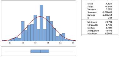
Carry out a log transformation (See Investigation 2.2, Question 9) and report the mean, median, and standard deviation of the transformed data. Verify that a log-normal probability model is reasonable for these data.
Mean (log turbidity): log NTU
Median (log turbidity): log NTU
Standard deviation (log turbidity): log NTU
Is a normal distribution reasonable for the log-transformed data?
3. Compare original and transformed statistics.
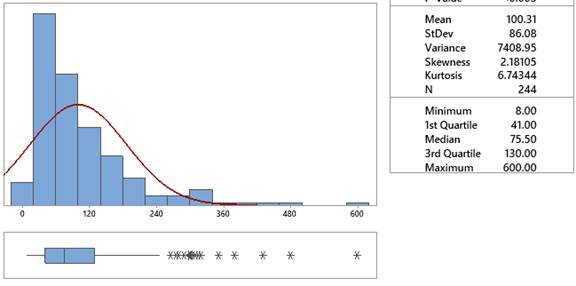
Consider the table of results
| Original scale | Ln of original values | Transformed scale |
|---|---|---|
| Mean = 100.3 | Ln(mean) = 4.608 | Mean(ln turbidity) = 4.301 |
| Median = 75.5 | Ln(median) = 4.324 | Median(ln turbidity) = 4.324 |
Are the mean and median values of the logged data values similar to each other? Is the mean of the logged turbidity values similar to the log of the mean of the turbidity values? Is the median of the logged turbidity values similar to the log of the median of the turbidity values?
Comparisons:
Solution.
The mean and median values of the transformed data are similar as we would expect with the transformed data now being symmetric.
The median turbidity value (before transforming) was 75.5. The natural log of this value is 4.3241. This is the same as the median of the log-turbidity values.
The mean turbidity value (before transforming) was 100.307. The natural log of this value is 4.6082, which is not the same as the mean of the log-turbidity values.
4. Explain median vs. mean transformation.
Explain why the median(log(turbidity)) is expected to be the same as log(median(turbidity)), but this interchangeability is not expected to work for the mean.
Solution.
We expect the medians to match because the median is essentially the middle value (slightly untrue with an even number of observations) and the same observation will still be the median value after the log transformation. However, the mean utilizes the numerical values and the relative distances between observations is changed with the log transformation.
5. Calculate confidence interval for transformed data.
Aside: Theory-Based Inference Applet.
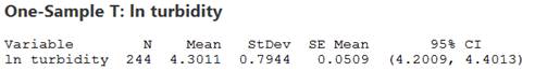
Use a one-sample t-confidence interval to estimate the mean of the log-turbidity value for this river.
6. Back-transform and interpret interval.
Discussion: Transformations and Back-Transformation.
Once you create a symmetric distribution, the mean and median will be similar. However, although transforming the data does not affect the ordering of the observations, it does impact the scaling of the values. So whereas the median of the transformed data is equal to taking the log of the median of the original data (at least with an odd number of observations), this does not hold for the mean. So when we back-transform our interval for the center of the population distribution, we will interpret this in terms of the median value rather than the mean value.
Study Conclusions.
A 95% confidence interval based on the transformed data equals (4.20, 4.40). Therefore, we will say we are 95% confident that the median turbidity in this river is between 66.69 NTU and 81.45 NTU, clearly less than the 150 NTU regulation. However, another condition for the validity of this procedure is that the observations are independent. Further examination of these data reveals seasonal trends. Adjustments need to be made to account for the seasonality before these data are analyzed.
Subsection 10.2.2 Practice Problem 2.8
Checkpoint 10.2.1. Calculate confidence interval for log response time.
Use the log transformation to calculate a 95% confidence interval for the mean log response time.
Checkpoint 10.2.3. Verify confidence interval procedure.
You have attempted of activities on this page.
