Investigation 2.4: The Ethan Allen

Section 9.1 Investigation 2.4: The Ethan Allen

Exercises 9.1.1 The Scenario

On October 2, 2005, the tour boat Ethan Allen capsized on Lake George in upstate New York. All 47 passengers on board were thrown into the lake, and 20 of them drowned. Although there were some claims that a large wave had hit the boat, an investigation by New York State Police (2006) concluded that the boat had been overloaded with heavy passengers.

🔗

Ethan Allen tour boat on Lake George

🔗

In fact, the average weight of the 47 passengers was found to be 174 pounds; whereas the boat was designed with the assumption that passengers would average 140 pounds.

🔗

1. Conjecture about weight distribution.

Do you think the distribution of the weights of 47 passengers might vary from boat to boat, even if they were randomly selected from the same (large) population of American adults?

🔗

Population distribution.

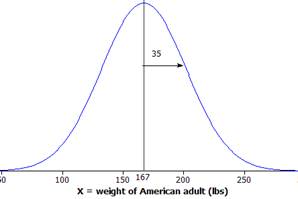
Data from the Centers for Disease Control and Prevention indicate that weights of American adults in 2005 had a mean of 167 pounds and a standard deviation of 35 pounds. (To convey that these are population values, we will use Greek letters to represent their values, \(\mu = 167\) and \(\sigma = 35\text{.}\))

🔗

If we also assume that the weight distribution has an approximately normal-shape, below is a possible outline of the distribution of the weights of the population of roughly 225 million adult Americans in 2005.

🔗

Possible population distribution of weights

Boat Weights.

Engineers estimated the maximum weight capacity of passengers that the Ethan Allen could accommodate to be 7500 pounds. If the tour boat company consistently accepted 47 passengers, what we want to know is the probability that the combined weight of the 47 passengers would exceed this capacity.

🔗

2. Identify observational units and variable for this research question.

Hint.

Notice that the probability of interest does not pertain to individual passengers.

🔗

The observational units are:

🔗

The variable is ,

🔗

Is the variable quantitative or categorical?

🔗

quantitative
categorical

Solution.

The observational units are the different boats (or boat trips) with 47 passengers each. The variable is the average weight of the 47 passengers on each boat. This variable is quantitative because it is measured on a numerical scale.

🔗

Instead of focusing on the total weight of the 47 passengers, we can instead work with the average weight of the 47 passengers.

🔗

3. Convert total weight to average weight.

Complete the following to indicate how these are equivalent:

🔗

Total weight of passengers is larger than 7500 lbs when average weight of 47 passengers is larger than: lbs.

🔗

Solution.

7500/47 = 159.574 pounds

🔗

So, to see how often the boat was sent out with too much weight, we need to know about the distribution of the average weight of 47 passengers from different boats (samples). Think about a distribution of sample mean weights from different random samples of 47 passengers, repeatedly selected from the population of adult Americans.

🔗

4. Center of sample means distribution.

Prediction: Where do you think the distribution of sample means will be centered?

🔗

pounds

🔗

5. Variability of sample means.

Do you think the distribution of sample means would have more variability, less variability, or the same variability as the distribution of weights of individual people?

🔗

More variability
Less variability
Same variability

🔗

6. Compare probabilities.

\(P(\text{average weight} > 159.6)\) \(P(\text{weight} > 159.6)\)

🔗

Hint.

🔗

larger
smaller
equal

🔗

Simulation Analysis.

To investigate this probability, we will generate random samples from a hypothetical population of adults’ weights. Open the WeightPopulations.txt data file and pretend each column is a different population of 20,000 adult tourists, each with a population mean weight (\(\mu\)) of 167 lbs and a population standard deviation (\(\sigma\)) of 35 lbs.

🔗

Using the Sampling from Finite Population applet (below or open in own window), carry out the following steps:

🔗

Press the Clear button.

🔗
Click inside the Paste population data box and type WeightPopulations.txt and press Use Data.
🔗

🔗
Once you see the data has loaded into the window, press Use Data (again).
🔗

🔗

🔗

7. Describe population distribution.

Describe the shape, mean (\(\mu\)), and standard deviation (\(\sigma\)) of pop1 (shown in the histogram under Population Data). You can also check the Show skewness box.

🔗

Solution.

The population is mound-shaped and symmetric (skewness statistic approx zero) with a mean (\(\mu\)) of 167 lbs and a standard deviation (\(\sigma\)) of 35 lbs.

🔗

Check the Show Sampling Options box. Keep the Number of Samples at 1 and specify the Sample Size to be 47 and press the Draw Samples button.
🔗

🔗
The weights for this random sample of 47 passengers from this population are displayed in blue and in the Most Recent Sample graph.
🔗

🔗

8. Describe sample distribution.

Describe the shape, center, and variability of this distribution. How does this sample distribution compare to the population distribution?

🔗

Most Recent Sample distribution:

Shape:

Mean:

Standard deviation:

Comparison (sample vs. population):

🔗

Notice that the mean of this sample (an \(\bar{x}\)) has also been added to the graph in the lower right Sampled Statistics graph.

🔗

Solution.

Results will vary but here is one example:

🔗

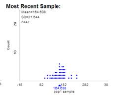
This simulated sample distribution is likely symmetric and bell-shaped with a mean similar to \(\mu\) and a standard deviation similar to \(\sigma\text{.}\)

🔗

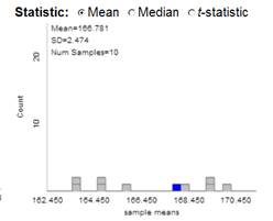
Press Draw Samples again. [Option: Scroll to the far right and check the "Vertical layout" box in the applet.]

🔗

9. Generate second sample.

Did you obtain the same sample of 47 weights? Did you obtain the same sample mean? Do either of the two sample means generated thus far equal the population mean?

🔗

Solution.

Probably obtained a different sample mean in the second sample.

🔗

Continue to press Draw Samples 8 more times (for 10 samples total), and notice the variability in the resulting sample means from sample to sample.

🔗

10. Generate 10 samples total.

Is a pattern beginning to emerge in the Sampled Statistics distribution graph?

🔗

Solution.

The values appear to be clustering around 167 but with less spread. Here is one example:

🔗

🔗

Now set the Number of Samples to 990 (for 1,000 total) and press Draw Samples.

🔗

11. Generate 1000 samples.

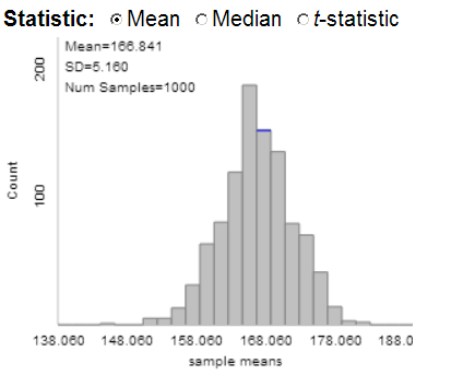
Describe the shape, center, and variability of the distribution of the sample means (lower right graph). How do these features compare to the population distribution? Which one of these features has changed the most vs. the population, and how has it changed?

🔗

Hint.

Note the change in scaling. You can check the Population scale box to rescale back to the original population scaling and add the location of the population mean.

🔗

Distribution of sample means (aka "sampling distribution"):

Shape:

Mean:

Standard deviation:

Comparison (sample means vs. population):

🔗

Solution.

Here is one example:

🔗

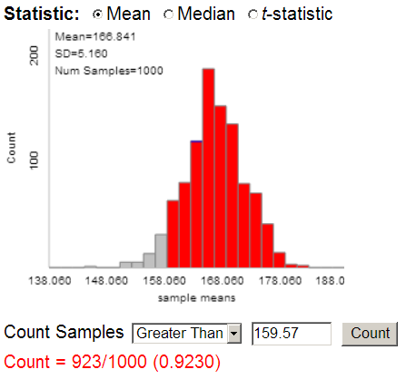
The shape should be approximately normal, similar to the population. The mean is 166.8, similar to \(\mu\) (167). The standard deviation is 5.16, much smaller than the value of \(\sigma\) for the population (35).

🔗

12. Use simulation for probability.

How can we use your simulated distribution of sample means to decide whether it is surprising that a boat with 47 passengers would exceed the (average) weight limit by chance (random sampling error) alone?

🔗

Solution.

We can count how many sample means are greater than the weight limit 159.57 lbs.

🔗

To count samples, specify the sample mean of interest (159.6) in the Count Samples box, use the pull-down menu to specify whether you want to count samples Greater Than, Less Than, or Beyond (both directions), then press Count.
🔗

🔗

13. Count samples exceeding limit.

To investigate the question posed in Question 11, what conclusions can you draw from the count displayed by the applet?

🔗

Solution.

We want to see how often we get a sample mean this larger or even larger, \(P(\bar{x} > 159.57)\text{.}\) Example results:

🔗

This indicates that over 92% of the time do we get an average weight above 159.57 (so above the weight limit for the boat) for a sample of 47 passengers.

🔗

Non-normal Population.

To carry out the preceding simulation analysis, we assumed that the population distribution had a normal shape. But what if the population of adult weights has a different, non-normal distribution? Will that change our findings?

🔗

Now choose the data from the second column (pop2) with the Choose variable pull-down menu on the left side.

🔗

14. Analyze skewed population.

Describe the shape of this population and what it means for the variable to have this shape in this context. How do the values of \(\mu\) and \(\sigma\) compare to the pop1 (rounding a bit)?

Shape:

Mean:

Standard deviation:

Comparison to previous population:

🔗

Solution.

The shape is skewed to the right (skew = 1.56). This would indicate most of the weights were on the lower end (120-200 lbs) but there can also be some much heavier adults in the population. The mean and standard deviation are the same as with population one (essentially).

🔗

Generate 1,000 random samples of 47 individuals from this population.

🔗
Sketch the distribution of sample means and note the values for the mean and standard deviation of the sampling distribution.

🔗

15. Sample from skewed population.

How does this distribution compare to the distribution in Question 11?

Mean:

SD:

Comparison:

Solution.

Example results:

🔗

Sampling distribution from skewed population

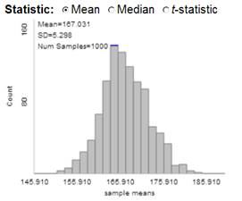
You should find that the shape is still approximately normal. The mean is still right around \(\mu\) (167) and the standard deviation is still right around 5.2.

🔗

Use the applet to approximate the probability of obtaining a sample mean weight of at least 159.574 lbs for a random sample of 47 passengers from population 2.

🔗

16. Probability for skewed population.

Has this probability changed considerably with the change in the shape of the distribution of the population of weights?

🔗

Solution.

We still find about 92% of the sample means above 159.57. Changing the population shape has not really changed our estimate of the probability.

🔗

Repeat this analysis using the other population distribution (pop3) in the data file and summarize your observations for the three populations in the table below.

🔗

17. Compare three populations.

Distribution of sample means comparison

🔗

Population	Shape (Skew)	Mean	Standard deviation
Normal
Skewed right
Uniform

Solution.

The distribution of sample means has not changed much with any of the changes in population shape.

🔗

Changing the Sample Size.

Now consider changing the sample size from 47 to 188 (four times larger).

🔗

18. Predict effect of larger sample size.

Predict how the shape, mean, and SD of the distribution of sample means would change (if at all).

🔗

In the applet, make this change of sample size from 47 to 188, and generate 1000 random samples (from the uniformly distributed population, pop3).

🔗

19. Test prediction with larger sample.

Did the shape of the sample means change very much? What about the mean of the sample means? What about the SD of the sample means? How were your predictions in Question 18?

🔗

Solution.

The shape and mean did not change but the standard deviation is much smaller, now around 2.5.

🔗

Discussion.

You should see that, as with the Investigation 1.12: Sampling Words, the shape of the population is not having much effect on the distribution of the sample means! In fact, you can show that the mean of the distribution of sample means from random samples is always equal to the mean of the population (any discrepancies you find are from not simulating enough random samples) and that, assuming the population is large compared to the size of the sample, the standard deviation of the distribution of sample means is equal to \(\sigma/\sqrt{n}\text{.}\) This standard deviation formula applies when the population size is large (more than 20 times the size of the sample) or infinite (so the randomly selected observations can be considered independent).

🔗

20. Explain standard deviation formula.

Explain why the formula for the standard deviation of the sample mean \((\sigma/\sqrt{n})\) makes intuitive sense (both the \(\sigma\) component and the \(\sqrt{n}\) component).

🔗

Solution.

\(\frac{\sigma}{\sqrt{n}}\) incorporates information from both the variability in the population itself and the sample size. If we have a variable with more person to person variability, we will also expect more sample to sample variability. If we have a larger sample size, we expect less sample to sample variability (the sample means will cluster more tightly around \(\mu\)).

🔗

Key Result: Central Limit Theorem.

If all possible samples of size \(n\) are selected from a large population or an infinite random process with mean \(\mu\) and standard deviation \(\sigma\text{,}\) then the sampling distribution of these sample means will have the following characteristics:

🔗

The mean will be equal to \(\mu\text{.}\)
🔗

🔗
The standard deviation will be equal to \(\sigma/\sqrt{n}\) (we can call this \(SD(\bar{x})\) or \(\sigma_{\bar{x}}\)).
🔗

🔗
Central Limit Theorem: The shape will be normal if the population distribution is normal, or approximately normal if the sample size is large regardless of the shape of the population distribution.
🔗

🔗

🔗

The convention is to consider the sample size large enough if \(n > 30\text{.}\) However, this rule really depends on the shape of the population. The more non-symmetric the population distribution, the larger the sample size necessary before the distribution of sample means is reasonably modeled by a normal distribution. You can use this table to change the sample size cut-off based on the value of the sample skewness.

🔗

Sample skewness	0.25	0.5	0.75	1.0	1.5	2.0
Minimum sample size	10	20	35	50	100	165

The population is considered large if it is more than 20 times the size of the sample.

🔗

Discussion.

In general, the shape of the distribution of sample means does not depend on the shape of the population distribution, unless you have small sample sizes. So if the population distribution itself follows a normal distribution, then we will always be willing to model the distribution of sample means with a normal distribution. However, we typically don’t know the distribution of the population (that’s why we need to collect data), but we can make a judgment based on the nature of the variable (e.g., biological characteristics, repeated measurements) or based on the information conveyed to us by the shape of the distribution of the sample data (e.g., normal probability plot).

🔗

In this example, a sample size of 47 appears large enough to result in a normal distribution for the distribution of sample means. However, you may have noticed a bit of a right skew when the population was skewed and in such a situation you would want a larger sample size before you were willing to model the distribution of sample means with a normal distribution.

🔗

Keep in mind that the results about the mean and standard deviation always hold for random samples: sample means cluster around the population mean and are less variable than individual observations! If the population size is not large, then a "finite population correction factor" can be applied as in Ch. 1.

🔗

21. Standardize the value.

Use the theoretical results for the mean and standard deviation of a sample mean to standardize the value of 159.57 lbs. [Hint: Start with a well-labeled sketch.] How might you interpret this value?

🔗

Solution.

\begin{equation*} \sigma / \sqrt{n} = 35/\sqrt{47} \approx 5.105 \end{equation*}

\begin{equation*} \frac{159.574 - 167}{5.105} = -1.45 \end{equation*}

🔗

22. Apply Central Limit Theorem.

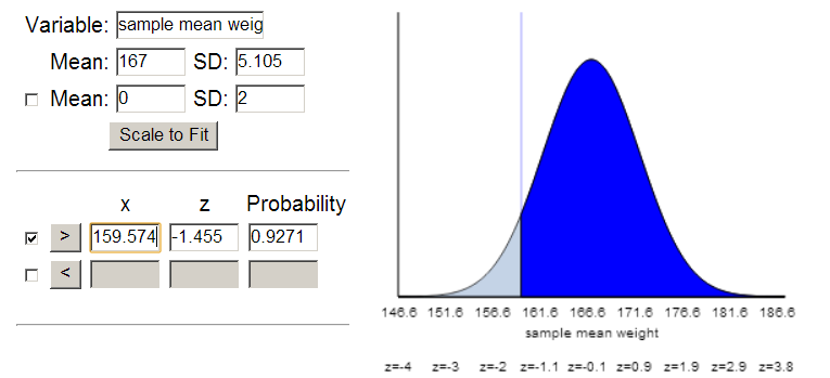
Use the result from the Central Limit Theorem and technology (e.g., the Normal Probability Calculator applet) to estimate the probability of a sample mean weight exceeding 159.57 lbs for a random sample of 47 passengers from a population with mean \(\mu = 167\) lbs and standard deviation \(\sigma = 35\) lbs. [Hint: Shade the area of interest in your sketch for Question 21.] How does this estimated probability compare to what you found with repeated sampling from the hypothetical populations?

🔗

Solution.

Using technology, we find \(P(\bar{x} > 159.57) = 0.9271\text{,}\) which is very close to what we found with the simulations (about 93%).

🔗

🔗

23. Identify concerns.

Identify one concern you might have with this analysis.

🔗

Hint.

What other assumption, apart from the shape of the population, was made in these simulations that may not be true in this study? Do you think this is a reasonable assumption for this study?

🔗

Solution.

We assumed the mean and standard deviation reported by the CDC in 2005 are accurate reflections of the weights of the passengers. This may or may not be the case.

🔗

Study Conclusions.

Assuming the CDC values for the mean and standard deviation of adult Americans’ weights, \(\mu = 167\) lbs and \(\sigma = 35\) lbs, we believe that the distribution of sample mean weights will be well modeled by a normal distribution (based both on the not extremely skewed nature of the variable and the moderately large sample size of 47, which is larger than 30). Therefore, the Central Limit Theorem allows us to predict that the distribution of \(\bar{x}\) is approximately normal with mean 167 lbs and standard deviation \(35/\sqrt{47} \approx 5.105\) lbs. From this information, assuming the CDC data is representative of the population of Ethan Allen travelers, we can estimate the probability of obtaining a sample mean of 159.57 lbs or higher to be 0.9264. Therefore, it is not at all surprising that a boat carrying 47 American adults capsized. In fact, the surprising part might be that it didn’t happen sooner!

🔗

Subsection 9.1.2 Practice Problem 2.4A

Checkpoint 9.1.1. Probability for 20 passengers.

Use the Sampling from Finite Population or the Central Limit Theorem to estimate the probability that the sample mean of 20 randomly selected passengers exceeds 159.57lbs, assuming a normal population with mean 167lbs and standard deviation 35lbs.

🔗

Checkpoint 9.1.2. Compare probabilities.

Is the probability you found in the previous question larger or smaller than the probability you found for 47 passengers? Explain why your answer makes intuitive sense.

🔗

Checkpoint 9.1.3. Uniform population.

Repeat the first question assuming a uniformly distributed population of weights. How do these two probabilities compare?

🔗

Hint.

Think about whether it is more appropriate to use the Sampling from Finite Population applet or the CLT to answer this question.

🔗

Checkpoint 9.1.4. Explain limitation.

Explain why the calculation in Checkpoint 9.1.1 does not estimate the probability of the Ethan Allen sinking with 20 passengers.

🔗

Subsection 9.1.3 Practice Problem 2.4B

Checkpoint 9.1.5. Finite population.

Use the Sampling from Finite Population applet or the Central Limit Theorem to estimate the probability that the sample mean of 47 randomly selected passengers would exceed 159.57lbs, assuming that random samples are repeatedly selected from a population of 80,000 individuals with mean 167 lbs and standard deviation 35 lbs. State any assumptions you need to make and support your answer statistically.

🔗

Subsection 9.1.4 Practice Problem 2.4C

Checkpoint 9.1.6. Explain averages.

In this investigation, we found that the average of the sample average is near the population average. Explain what each use of the term "average" means in this statement.

🔗

You have attempted of activities on this page.

🔗

Prev Top Next