A model is an artificial representation or a simplification of something more complicated, like a toy airplane. Models can be useful in making predictions (e.g., weather models) or to help us better understand the phenomena under study. For example, what factors impact the severity of a hurricane?
Descriptions will vary. For example: Warm water is essential to fuel the storm. When humid air goes up, rainfall occurs, helping hurricanes form. If the speed of upper wind in a certain area is too fast, hurricanes won’t form. If the upper wind levels are calmer, this creates a more likely environment for a hurricane to form.
Opinions will vary. We could compare the predictions to recent data to see how well they match up. If the results don’t match up, we could gather more data in order to improve the model. This could include additional variables we haven’t considered yet.
In this course, you will encounter two main types of models: statistical models and probability/simulation models. For example, the Random Babies simulation in Investigation B, allowed you to simulate hypothetical data to estimate probabilities of different events. As long as the model valid, we can predict that all four mothers receiving the correct babies would not happen very often in the long run. Most models rely on simplifying assumptions, like babies being returned “completely at random.”
Histograms bin the observations rather than trying to represent each individual value. They are more useful in looking at the overall distribution for a larger number of observations.
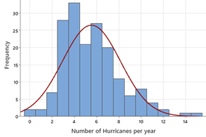
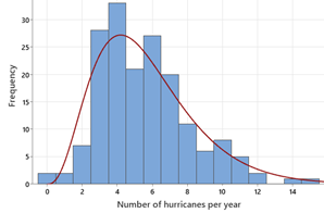
The curve on the left is more symmetric whereas the curve on the right has a right skewedness to it. The right skew appears to better match up with the histogram.
By "model," we are looking for a simpler representation of the general pattern in the histogram. A mathematical model can then be used to make predictions about future observations, as long as the "process" is not changing. In particular, while we didn’t observe a year with 13 hurricanes, the model would predict that could happen, but rarely.
We suspect not everyone will find the same exact measurement. There could be different measurement techniques, different lighting at the time of the measurement, different tennis balls.
We can think of these measurements as observations from a random process, which we can summarize with a statistical model. If we consider 28.5cm the “true value,” then we can write our statistical model as
Again, the model is a simpler representation of the measurement process. This would help us make predictions or identify observations that seem way different from what we might expect due to more typical measurement errors.
Researchers often compare data generated from a model to observed data to help validate the model. If the model’s data reasonably matches the observed data, that helps confirm that they (the model builders) understand the underlying data generating process.
Suggest and label four possible sources of variation in the tennis ball measurements. Make each source of variation one of the pie charts and conjecture error magnitudes and probabilities for each source (e.g., right now, Spinner 1 assumes a perfect measurement with 0.50 probability, a -0.10 cm error with 0.25 probability and a +0.10 cm error with 0.25 probability). Describe your model below.
Simulate one measurement by pressing the Simulate data button. What did you find for the total random error across your four sources? Will this be the same every time?
Checkpoint1.3.4.Compare Simulated to Observed Data.
Generate the same number of measurements as we took in class. Compare the simulated data to the actual data from class (e.g., shape, center, spread). What looks similar and what looks different?
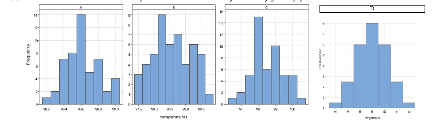
Suppose human body temperatures can be modelled with a normal distribution with mean 98.6°F. Suppose you take repeated measures of your temperature over several days.
Distributions A-C have the same mean (98.6) but different spread or variability. Which of the graphs above has the largest standard deviation? Approximate the value of each standard deviation by interpreting the standard deviation as a “typical” deviation from the mean.
Checkpoint1.3.10.Evaluate Distribution Assumptions.
The 4 distributions are all roughly “bell-shaped and symmetric.” Do you think actual repeated body measurements on the same individual will behave this way? Briefly explain your reasoning.
Suppose I randomly select one of the temperatures from Distribution C. Approximate the probability that the temperature is larger than 99°F. Interpret your probability in context.