Investigation 3.5: Dolphin Therapy

Section 12.1 Investigation 3.5: Dolphin Therapy

Antonioli and Reveley (2005) investigated whether swimming with dolphins was therapeutic for patients suffering from clinical depression. The researchers recruited 30 subjects aged 18-65 with a clinical diagnosis of mild to moderate depression through announcements on the internet, radio, newspapers, and hospitals in the U.S. and Honduras. Subjects were required to discontinue use of any antidepressant drugs or psychotherapy four weeks prior to the experiment, and throughout the experiment. These 30 subjects went to an island off the coast of Honduras, where they were randomly assigned to one of two treatment groups. Both groups engaged in one hour of swimming and snorkeling each day, but one group (Dolphin Therapy) did so in the presence of bottlenose dolphins and the other group (Control) did not. At the end of two weeks, each subject’s level of depression was evaluated, as it had been at the beginning of the study, and each subject was categorized as experiencing substantial improvement in their depression symptoms or not. (Afterwards, the control group had 1-day session with the dolphins.)

🔗

Checkpoint 12.1.1. Identify Study Components.

Identify the observational units and variables in this study. Also indicate which variable is being considered the explanatory variable and which the response variable.

🔗

Observational units:

🔗

Explanatory variable:

🔗

Response variable:

🔗

Solution.

Observational units: 30 subjects with clinical depression

🔗

Explanatory variable: Treatment group (dolphin therapy or control)

🔗

Response variable: Whether or not the subject showed substantial improvement

🔗

Checkpoint 12.1.2. Study Type.

Was this an observational study or an experiment? Explain how you are deciding.

🔗

Solution.

This was an experiment because the researchers randomly assigned subjects to the treatment groups (dolphin therapy vs. control).

🔗

The following two-way table summarizes the results of this experiment:

🔗

Table 12.1.3.

🔗

	Dolphin Therapy	Control Group	Total
Showed substantial improvement	10	3	13
Did not show substantial improvement	5	12	17
Total	15	15	30

🔗

Checkpoint 12.1.4. For Practice.

What proportion of all subjects showed substantial improvement?

🔗

What proportion of subjects who were given dolphin therapy improved?

🔗

Solution.

Overall: 13/30 = 0.433

🔗

Dolphin therapy: 10/15 = 0.667

🔗

Checkpoint 12.1.5. Calculate Difference in Proportions.

Calculate the conditional proportion of substantial improvement for the dolphin therapy group:

🔗

Calculate the conditional proportion of substantial improvement for the control group:

🔗

Calculate the difference in the conditional proportions (dolphin therapy - control):

🔗

Solution.

Dolphin therapy: 10/15 = 0.667; Control: 3/15 = 0.200; Difference: 0.667 - 0.200 = 0.467

🔗

Checkpoint 12.1.6. Initial Assessment.

Do the data appear to support the claim that dolphin therapy is more effective than the control program?

🔗

Solution.

Yes, a much higher proportion improved in the dolphin therapy group (66.7%) compared to the control group (20%).

🔗

Checkpoint 12.1.7. Alternative Explanation.

Suppose swimming with dolphins is no more effective than swimming alone. What could be another possible explanation for the difference in these two sample proportions?

🔗

Solution.

Random chance from the random assignment process could have placed more of the people who were going to improve anyway into the dolphin therapy group.

🔗

We must ask the same questions we have asked before – is it possible that this difference has arisen by random chance alone if there was no effect of the dolphin therapy? If so, how surprising would it be to observe such an extreme difference between the two groups?

🔗

One way to define a parameter in this case is to let \(\pi_{dolphin} - \pi_{control}\) denote the difference in the underlying probability of substantial improvement between the two treatment conditions.

🔗

Checkpoint 12.1.8. State Hypotheses.

State appropriate null and alternative hypotheses to reflect the researchers’ conjecture in terms of this parameter.

🔗

\(H_0\text{:}\)

🔗

\(H_a\text{:}\)

🔗

Solution.

\(H_0\text{:}\) \(\pi_{dolphin} - \pi_{control} = 0\) (no difference in probability of improvement)

🔗

\(H_a\text{:}\) \(\pi_{dolphin} - \pi_{control} > 0\) (dolphin therapy has higher probability of improvement)

🔗

Checkpoint 12.1.9. Design Simulation.

So under the null hypothesis, we are assuming that there is no difference in the treatment effect between the two treatments. In other words, whether or not people improved is not related to which group they are put in. Explain how you could design a simulation to help address this question, keeping in mind that this study involved random assignment not random sampling. Also keep in mind that this simulation will assume the null hypothesis is true.

🔗

Solution.

We could assume that 13 of the 30 people were going to improve regardless of treatment, and 17 were not going to improve. Then we could randomly assign these 30 people to the two groups (15 in each) many times and see how often we get a difference as large as 0.467 or larger.

🔗

One way to model this situation is by assuming 13 of the 30 people were going to demonstrate substantial improvement regardless of whether they swam with or without dolphins. Then the key question is how unlikely is it for the random assignment process alone to randomly place 10 or more of these 13 improvers into the dolphin therapy group (that is, a difference in the conditional proportions that improve of 0.467 or larger)? If the answer is that this observed difference would be very surprising if the dolphin and control therapies were equally effective, then we would have strong evidence to conclude that dolphin therapy is more effective.

🔗

Checkpoint 12.1.10. Physical Simulation.

To model the chance variability inherent in the random assignment process, under the null hypothesis, take a set of 30 playing cards or index cards, one for each participant in the study. Designate 13 of them to represent improvements (e.g., red suited cards, blue colored index cards, or S-labeled index cards) and then mark 17 of them to represent non-improvements (e.g., black suited cards, green colored index cards, or F-labeled index cards). Shuffle the cards and deal out two groups: 15 of the "subjects" to the dolphin therapy group and 15 to the control group. Complete the following two-way table to show your "could have been" result under the null hypothesis.

🔗

Simulation Repetition #1:

🔗

Table 12.1.11.

🔗

	Dolphin Therapy	Control Group	Total
Showed substantial improvement			13 (blue)
Did not show substantial improvement			17 (green)
Total	15	15	30

Also calculate the difference in the conditional proportions (dolphin – control) from this first simulated repetition, and indicate whether this simulated result is as extreme as the observed result:

🔗

Solution.

Results will vary.

🔗

Checkpoint 12.1.12. Additional Repetitions.

Repeat this hypothetical random assignment two more times and record the "could have been" tables:

🔗

Repetition 2:

🔗

Table 12.1.13.

🔗

	Dolphin	Control
Yes
No

Repetition 3:

🔗

Table 12.1.14.

🔗

	Dolphin	Control
Yes
No

Note: You may have noticed that once you entered the number of improvers in the Dolphin Group into the table, the other entries in the table were pre-determined due to the "fixed margins." So for our statistic, we could either report the difference in the conditional proportions or the number of successes (improvers) in the Dolphin group as these give equivalent information.

🔗

Solution.

Results will vary.

🔗

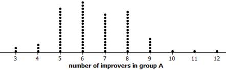
Pool your results for the number of successes (blue index cards) assigned to the Dolphin Group for your 3 repetitions with the rest of your class and produce a well-labeled dotplot of the null distribution.

🔗

Checkpoint 12.1.15. Interpret Dotplot.

What does each dot in the above graph represent?

🔗

Hint.

Think about what you would have to do to add another dot to the graph. How should you label the horizontal axis?

🔗

Solution.

Each dot represents one simulated random assignment of the 30 subjects to the two groups, showing the number of improvers that ended up in the dolphin therapy group. The horizontal axis should be labeled "Number of improvers in dolphin therapy group."

🔗

Example results from pooling class data:

🔗

Checkpoint 12.1.16. Preliminary Assessment.

Granted, we have not done an extensive number of repetitions, but how’s it looking so far? Does it seem like the actual experimental results (the observed 10/3 split) would be surprising to arise purely from the random assignment process under the null hypothesis that dolphin therapy is not effective? Explain.

🔗

Solution.

Results will vary, but students should notice that getting 10 or more improvers in the dolphin group appears to be unusual/rare.

🔗

We really need to do this simulated random assignment process hundreds, preferably thousands of times. This would be very tedious and time-consuming with cards, so let’s turn to technology.

🔗

Open the Dolphin Study applet.

🔗

Confirm that the two-way table displayed by the applet matches that of the research study.

🔗
Check Show Shuffle Options and confirm that there are 30 total "people": 13 blue and 17 green.

🔗
Press Shuffle.

🔗

🔗

Watch as the applet repeats what you did: Shuffle the 30 cards and deal out 15 for the "Dolphin therapy" group, separating blue cards (successes) from green cards (failures), and 15 for the "Control Group"; create the table of "could have been" simulated results; add a dot to the dotplot for the number of improvers (blue cards) randomly assigned to the "Dolphin therapy" group (GroupA successes).

🔗

Checkpoint 12.1.17. Applet Exploration.

Now press Shuffle four more times. Does the number of successes vary among the repetitions?

🔗

Solution.

Yes, the number of successes in the dolphin group varies from repetition to repetition.

🔗

Checkpoint 12.1.18. Null Distribution.

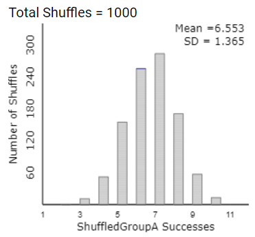
Enter 995 for the Number of shuffles. This produces a total of 1,000 repetitions of the simulated random assignment process under the null hypothesis (the "null distribution" or a "randomization distribution"). What is the value of the mean of this null distribution? Explain why this center makes intuitive sense.

🔗

Solution.

The mean should be around 6.5. This makes sense because if we randomly assign 15 of the 30 subjects to the dolphin group, we would expect about half of the 13 improvers (6.5) to end up in that group on average.

🔗

Example results:

🔗

Checkpoint 12.1.19. Compare to Observed Result.

Now we want to compare the observed result from the research study to these "could have been" results under the null hypothesis.

🔗

How many improvers were there in the Dolphin therapy group in the actual study?

🔗

Based on the resulting dotplot, does it seem like the actual experimental results would be surprising to arise solely from the random assignment process under the null hypothesis that dolphin therapy is not effective? Explain.

🔗

Solution.

There were 10 improvers in the dolphin therapy group. Yes, this appears to be in the upper tail of the distribution, suggesting it would be surprising to get this result by chance alone.

🔗

Checkpoint 12.1.20. Calculate p-value.

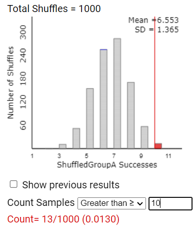
In the Count Samples box, enter the observed statistic from the actual study and press Count to have the applet count the number of repetitions with 10 or more successes in the Dolphin group. In what proportion of your 1000 simulated random assignments were the results as (or more) extreme as the actual study?

🔗

Solution.

The p-value should be approximately 0.02 to 0.04 (will vary slightly due to randomness).

🔗

Checkpoint 12.1.21. Difference in Proportions.

We said above that it would be equivalent to look at the difference in the conditional proportions. Use the Statistic pull-down menu to select Difference in proportions.

🔗

How does the null distribution (including the mean) change?

🔗

Does this make sense?

🔗

How would you estimate the p-value now?

🔗

How does the p-value change?

🔗

Solution.

The null distribution is now centered at 0 (since we expect no difference under the null hypothesis). The shape is similar but the scale has changed. The p-value is estimated by counting how many repetitions have a difference of 0.467 or larger, and should be approximately the same as before.

🔗

Checkpoint 12.1.22. Interpret p-value.

Interpret the p-value you found.

🔗

Hint.

Same reasoning as in Investigation 3.1, but now also focus on the source of randomness that was modelled in the simulation.

🔗

Solution.

The p-value represents the probability of obtaining a difference in proportions as large as 0.467 (or 10 or more improvers in the dolphin group) purely by chance from the random assignment process, assuming that dolphin therapy has no effect on improvement.

🔗

Checkpoint 12.1.23. Strength of Evidence.

Is this empirical p-value small enough to convince you that the experimental data that the researchers obtained provide strong evidence that dolphin therapy is effective (i.e., that the null hypothesis is not correct)?

🔗

Solution.

Yes, a p-value between 0.01 and 0.05 provides moderate to strong evidence against the null hypothesis, suggesting that dolphin therapy is effective.

🔗

Checkpoint 12.1.24. Confounding Variables.

Is it reasonable to attribute the observed difference in success proportions to the dolphin therapy, or could the difference be due to a confounding variable? Explain.

🔗

Solution.

Yes, it is reasonable to attribute the difference to dolphin therapy because this was a randomized experiment. Random assignment tends to balance out potential confounding variables between the two groups.

🔗

Checkpoint 12.1.25. Generalizability.

To what population is it reasonable to generalize these results? Justify your answer.

🔗

Solution.

Because this was not a random sample, we should be cautious about generalizing beyond people similar to those who volunteered for this study – people aged 18-65 with mild to moderate depression who could afford to travel to Honduras for two weeks.

🔗

Discussion.

This procedure of randomly reassigning the response variable outcomes to the explanatory variable groups is often called a "randomization test." The goal is to assess the chance variability from the random assignment process (as opposed to random sampling), though it is sometimes used to approximate the random chance arising from random sampling as well. Use of this procedure models the two-way table with fixed row and column totals (e.g., people were going to improve or not regardless of which treatment they received).

🔗

Study Conclusions.

Due to the small p-value (0.01 < p-value < 0.05) from our "randomization test," we have moderately strong evidence that "luck of the draw" of the random assignment process alone is not a reasonable explanation for the higher proportion of subjects who substantially improved in the dolphin therapy group compared to the control group. Thus the researchers have moderate evidence that subjects aged 18–65 with a clinical diagnosis of mild to moderate depression (who would apply for such a study and fit the inclusion criteria) will have a higher probability of substantially reducing their depression symptoms if they are allowed to swim with dolphins rather than simply visiting and swimming in Honduras. Because this was a randomized comparative experiment, we can conclude that there is moderately strong evidence that swimming with dolphins causes a higher probability of experiencing substantial improvement in depression symptoms. But with this volunteer sample, we should be cautious about generalizing this conclusion beyond the population of people suffering from mild-to-moderate depression who could afford to take the time to travel to Honduras for two weeks.

🔗

Subsection 12.1.1 Practice Problem 3.5A

A 2010 study compared two groups: One group was reminded of the sacrifices that physicians have to make as part of their training, and the other group was given no such reminder. All physicians in the study were then asked whether they consider it acceptable for physicians to receive free gifts from industry representatives. It turned out that 57/120 in the "sacrifice reminders" group answered that gifts are acceptable, compared to 13/60 in the "no reminder" group.

🔗

Checkpoint 12.1.26. Identify Variables.

Identify the explanatory and response variables in this study.

🔗

Checkpoint 12.1.27. Random Assignment.

Do you believe this study used random assignment? What would that involve?

🔗

Checkpoint 12.1.28. Random Sampling.

Do you believe this study used random sampling? What would that involve?

🔗

Checkpoint 12.1.29. Simulation Analysis.

Explain how you would carry out a simulation analysis to approximate a p-value for this study.

🔗

Hint.

How many cards? How many of each type? How many would you deal out? What would you record? How would you find the p-value?

🔗

Checkpoint 12.1.30. Unequal Sample Sizes.

A colleague points out that the sample sizes are not equal in this study, so we can’t draw meaningful conclusions. How should you respond?

🔗

Subsection 12.1.2 Practice Problem 3.5B

Checkpoint 12.1.31. Two-Sided p-value.

How would you find a two-sided p-value for the dolphin study?

🔗

You have attempted of activities on this page.

🔗

Prev Top Next