ISCAM: Investigating Statistical Concepts, Applications, and Methods

Analyzing the differences:

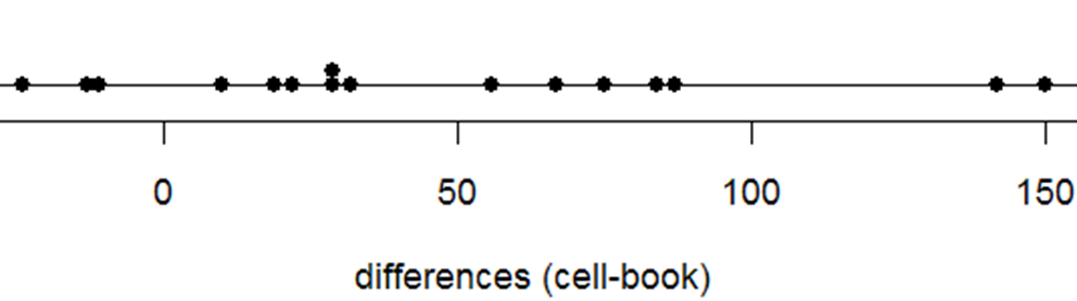
The sample mean difference in reaction times (cell minus control) is \(\bar{x}_{diff} = 47.125\) milliseconds, with a standard deviation of \(s_d = 51.331\) milliseconds. The dotplot reveals that most of the differences are positive, suggesting that subjects talking on a cell phone tend to take longer to react than subjects listening to a book-on-tape.

The null hypothesis says that the mean reaction time is the same among cell phone users as among book-on-tape listeners (\(H_0: \mu_{cell} - \mu_{control} = 0\)). The alternative says that the mean reaction time is larger among cell phone users than among book-on-tape listeners (\(H_a: \mu_{cell} - \mu_{control} > 0\)).

We can carry out the simulation easily with the Matched Pairs applet or with R.

Copying and pasting the data into the Matched Pairs applet with 1,000 repetitions we get the results shown here:

Using R to carry out the simulation instead:

MeanDiffs=0
for (i in 1:10000){
  multiplier=sample(c(-1,1), 16, replace=TRUE)
  RandomizedData=differences*multiplier
  MeanDiffs[i]=mean(RandomizedData)
}

From R: The empirical p-value is the proportion of these 10,000 repetitions in which the mean difference is 47.125 or more, because 47.125 is the value of the sample mean difference from the actual experimental data. None of the 10,000 repetitions produced such a large mean difference, so the empirical p-value is 0. The simulation therefore shows that we would almost never get a result as extreme as the actual experiment did, if there were really no difference between reactions to cell phone vs. book-on-tape, so we have extremely strong evidence that the cell phone really does increase reaction times.

Because the sample size (16) is fairly small, the t-procedures are valid only if the population of differences follows a normal distribution. The dotplot of differences from these 16 subjects looks roughly symmetric, so the t-procedures are probably valid to apply here.

The standardized statistic is \(t = \frac{\bar{x}_{diff} - 0}{s_{diff}/\sqrt{n_{diff}}} = \frac{47.125}{51.331/\sqrt{16}} \approx 3.67\text{.}\) The p-value is the probability that a t-distribution with 15 degrees of freedom is 3.67 or larger; R reveals this p-value to be 0.001137. This p-value is very small, so we would reject the null hypothesis at the 0.05 and 0.01 significance levels. The experimental data provide very strong evidence that talking on a cell phone does cause an increase in mean reaction time, as compared to listening to a book-on-tape. The cause/effect conclusion is justified because this is a randomized experiment with a very small p-value.

Note: This evidence is stronger than what we saw with the sign test in Example 2.2.

A 95% confidence interval for the population mean difference \(\mu_d\) is:

which is \(47.125 \pm 2.131 \times \frac{51.331}{\sqrt{16}}\text{,}\) which is \(47.125 \pm 27.347\text{,}\) which is \((19.778, 74.472)\text{.}\)

We can be 95% confident that the mean reaction time while talking on a cell phone is between roughly 20 and 75 milliseconds longer than when listening to a book-on-tape.

A 95% prediction interval for the difference in reaction times for a particular subject is:

which is \(47.125 \pm 2.131 \times 51.331\sqrt{1 + \frac{1}{16}}\text{,}\) which is \(47.125 \pm 112.753\text{,}\) which is \((-65.628, 159.878)\text{.}\)

We can be 95% confident that an individual subject will react anywhere from 65 milliseconds more quickly to 160 milliseconds more slowly talking on a cell phone as compared to listening to a book-on-tape.

An advantage of the sign test from Chapter 2 is we don’t need to rely on large sample sizes or normality of the differences for the procedure to be valid. However, by ignoring some information in the data, we would expect this procedure to have lower power and we lose information about the size of the difference. The conditions for the t-procedure seem to be satisfactorily met here.