
Section 19.1 Comparing Groups

In this investigation, you will consider how to compare two groups on a quanttiative response. Then you will take a detour to learn about the details of "two-sample t-procedures" for inference about the difference in means between two groups.

Exercises 19.1.1 Investigation 4.2: The Elephants in the Room

Researchers Holdgate et al. (2016) studied walking behavior of elephants in North American zoos to see whether there is a difference in average distance traveled by African and Asian elephants in captivity. They put GPS loggers on 33 African elephants and 23 Asian elephants, and measured the distance (in kilometers) the elephants walked per day.
Introduction image for Investigation 4.2

1. Identify Study Components.

Identify the observational units and variable of interest. Is the variable quantitative or categorical? Which graphs and numbers might you use to compare these two species?
Solution.
Observation units = 56 elephants, Variable = How many km did the elephant walk per day? This is a quantitative variable. We could look at dotplots, boxplots, histograms, means/SDs, five number summaries in order to compare the walking distances.
Open the elephants.txt data file. First, look at the data by creating a graph of distances separated by species. When using graphs to compare groups it is especially important that comparative graphs be drawn on the same scale. Note: These data are stacked as each column is a different variable (species and distance).

2. Create Comparative Graphs.

Use technology (Applet, R, or JMP) to create comparative graphs of walking distances by species. Choose one set of instructions below by clicking on a hint.
Hint 1. Descriptive Statistics applet
Use the Descriptive Statistics applet to create comparative graphs:
  • Copy the data to the clipboard. In the applet, check the Stacked box. Press Clear and paste the data into the Sample data window and press Use Data. (Or type elephants.txt in the empty Paste data window.) (Or use this link and press the Use Data button.)
  • Use the Separate by pull-down menu to select the Species categorical variable
  • You have radio button options for Histograms and Boxplots.
Hint 2. R/Sage Instructions
Use R to create comparative graphs:
Hint 3. JMP Instructions
Use JMP to create comparative graphs:
  • Choose Analyze > Distribution and specify both the quantitative variable (Y, Columns) and the categorical variable (By).
  • Press OK.
  • Use the Distributions hot spot to select Stack.
  • (See also File > Preferences)
JMP dialog for casting columns into roles
OR
  • Select Graph > Graph Builder.
  • Drag Distance to the X axis and Species to the Y axis.
  • Use the icons across the top to change to boxplots and histograms.
  • Press Done to complete the graph.
  • See also Analyze > Tabulate.
JMP Graph Builder icons for boxplots and histograms
Note: When comparing groups, some boxplot displays vary the other dimension of the box size by relative sample size.

3. Identify Outliers.

According to the boxplots, were there any “outlier” elephants? Explain how you know.
Hint.
Outliers are typically shown as individual points beyond the whiskers of the boxplot.
Solution.
Yes, there appear to be outliers in both groups. The boxplot will show these as individual points beyond the whiskers, indicating elephants that walked unusually long or short distances compared to others in their group.

4. Limitation of Boxplots.

What is a limitation to using only boxplots to compare these two distributions?
Hint.
Think about what information boxplots show versus what they hide about the distribution.
Solution.
Boxplots only show summary statistics (median, quartiles, range) and outliers. They don’t show the actual shape of the distribution, the number of observations at different values, or whether there are multiple modes. Dotplots or histograms provide more detailed information about the distribution’s shape.

5. Compare Distributions.

Explore the differences in the walking distances between the African and Asian elephants. Which species tended to walk more? Which species showed greater variability? Which distribution is more symmetric?
Hint.
Look at the centers, spreads, and shapes of the two distributions.
Solution.
African elephants tended to walk more on average (higher center). Asian elephants showed greater variability (wider spread). The Asian elephant distribution appears more symmetric, while the African elephant distribution may be slightly skewed.
And we can calculate separate summary statistics for the two species.

6. Calculate Numerical Summaries.

Use technology (Applet, R, or JMP) to calculate numerical summaries for each species. Choose one set of instructions below by clicking on a hint.
Hint 1. Descriptive Statistics applet
Check the Mean: Actual and Std dev: Actual boxes (at least)
Hint 2. R/Sage Instructions
Use R to calculate numerical summaries:
Hint 3. JMP Instructions
Use JMP to calculate numerical summaries:
  • Choose Analyze > Distribution and specify both the quantitative variable (Y, Columns) and the categorical variable (By).
  • Press OK.
  • Use the Distributions hot spot to select Stack.

7. Record Summary Statistics.

Determine the sample sizes, sample means, and the sample standard deviations for each group and record these below, using appropriate symbols.
Summary Statistics for Elephant Walking Distances
Species n Mean SD
African 
Asian

8. Predict Statistical Significance.

Do you think the difference in sample means is going to be statistically significant? What does statistical significance mean in this context? (What null and alternative hypotheses can we test?)
Before we can address statistical significance, we need more information as to how much we expect a difference in sample means to vary from sample to sample (e.g., what if we had lots of different zoos, each with random samples of each type of elephant). We will take a detour to explore this in a case where we have the populations to begin with to see some rather familiar results.

9. Outline Simulation Steps.

Outline the simulation steps we need to use.

Exercises 19.1.2 Probability Detour: Sampling Distribution of Difference in Two Means

To understand how differences in sample means behave, let’s explore a hypothetical scenario where we know the population distributions...
The file NBASalaries2025.txt contains season salaries (in millions of dollars) for all NBA basketball players at the start of the 2025-26 season (downloaded from ESPN NBA salaries July 2025). Players without a team affiliation or without a listed salary were not included in the data set.

1. Salary Distribution Shape.

Do you expect salary data to be symmetric or skewed, and if skewed, in which direction? Explain.

2. Mean vs Median.

Which do you suspect will be larger, the mean or median salary? Explain.
Sampling from Two Populations applet
  • Use the Select data pull-down menu to choose NBA Salaries (2025)
  • Press Use Data to load the Salary and Conference population data into the applet.

3. Population Parameters.

Record the population sizes, means, and standard deviations for the Western and Eastern conferences.
League Count Mean SD
Western  
Eastern
What symbols can we use to represent these values?
Are the shapes of the distributions as you expected?
Hint.
Use the applet to find the population parameters from the data file.
Solution.
The population sizes are approximately \(N_{\text{West}}\)=243 Western and \(N_{\text{East}}\)=229 Eastern players. The mean salaries are approximately \(\mu_{\text{West}} = 11.7\) million dollars and \(\mu_{\text{East}} = 11.3\) million dollars. The standard deviations are approximately \(\sigma_{\text{West}} = 13.8\) million dollars and \(\sigma_{\text{East}} = 13.3\) million dollars. Both distributions are strongly right-skewed as expected for salary data.
Select a random sample of 20 players from each conference:
  • Check the Show Sampling Options box. (You may have to scroll right in ther applet.)
  • Specify sample sizes of 20 for each sample and press Draw Samples.
  • Select the Plot radio button.

4. Sample Statistics.

Record the sample means and sample standard deviations for your samples.
Sample Statistics for NBA Salaries by Conference
League n Mean SD
Western  
Eastern  
How do the sample results compare to the population results? What about the shapes of the samples?
Hint.
Compare your sample statistics to the population parameters recorded earlier.
Solution.
Sample results will vary, but the sample means should be reasonably close to the population means, and the sample standard deviations should be reasonably close to the population standard deviations. The sample distributions may appear less skewed than the population distributions due to smaller sample sizes.
Repeat this process many times (at least 1000) to generate a sampling distribution of the difference in sample means (East - West).
  • Enter 1000 (or more) for the Number of samples.
  • Press Sample.

5. Generate Sampling Distribution.

Examine the distribution of differences in sample means.
Hint.
Generate at least 1000 samples to see the shape of the sampling distribution.
Solution.
After generating 1000+ samples, you should see a distribution of differences in sample means that is approximately normal, centered near the difference in population means (about 0.4 million).

6. Shape of Distribution.

Describe the shape of the sampling distribution of the difference in sample means. How does the distribution of the differences in sample means compare to the shape of the salary distributions themselves?
Hint.
Compare the shape of this distribution to the original population distributions.
Solution.
The sampling distribution of the difference in sample means is approximately normal (symmetric, bell-shaped), even though the individual salary distributions are strongly right-skewed. This illustrates the Central Limit Theorem for differences in means.

7. Center of Distribution.

What is the approximate center of the sampling distribution? Is this what you expected?
Solution.
The center is approximately at the difference in population means (\(\mu_{\text{East}} - \mu_{\text{West}} \approx -0.4\) million). This is expected because the difference in sample means is an unbiased estimator of the difference in population means.

8. Variability.

But of course, what you really want to know about is the variability. Is there more or less variability in this distribution compared to the variability in each population?
Solution.
There is much less variability in the sampling distribution of the difference in sample means compared to the variability in each population. This is because we are averaging values, which reduces variability.

9. Predicted Standard Error.

We know there should be less variability because we are talking about sample means rather than individual observations. But how much variability do we expect to find in the distribution of sample means taken from the Western conference? What about the Eastern conference? Is the variability in the difference in sample means larger or smaller than in the individual distributions?
Solution.
For Western conference: \(\sigma_{\bar{x}_{\text{West}}} = \sigma_{\text{West}}/\sqrt{n} = 13.8/\sqrt{20} \approx 3.09\) million.
For Eastern conference: \(\sigma_{\bar{x}_{\text{East}}} = \sigma_{\text{East}}/\sqrt{n} = 13.3/\sqrt{20} \approx 2.97\) million.
The variability in the difference would be approximately \(\sqrt{3.09^2 + 2.97^2} \approx 4.28\) million, which is smaller than the individual population standard deviations but larger than either individual standard error.

Key Result: Sampling Distribution of Difference in Two Means.

A theorem similar to the Central Limit Theorem indicates that if we have two infinite, normally distributed populations, with means \(\mu_1\) and \(\mu_2\) and standard deviations \(\sigma_1\) and \(\sigma_2\text{,}\) and we take independent random samples from each population, the sampling distribution of \(\bar{x}_1 - \bar{x}_2\) will follow a normal distribution with mean \(\mu_1 - \mu_2\) and standard deviation \(\sqrt{\sigma_1^2/n_1 + \sigma_2^2/n_2}\text{.}\)
This is a nice theoretical result, but we seldom meet these conditions exactly.

10. Summary of Results.

Summarize your findings about the distribution of the difference in sample means (shape, center, spread) and compare to the theoretical predictions.
Hint.
Compare what you observed in the simulation to the Key Result above.
Solution.
Shape: The sampling distribution is approximately normal, even though the populations are skewed. Center: Approximately \(\mu_{\text{East}} - \mu_{\text{West}} \approx -0.4\) million. Spread: Standard deviation approximately 4.3 million, which matches the theoretical prediction \(\sqrt{13.8^2/20 + 13.3^2/20} \approx 4.28\) million.

11. Violations of Assumptions.

Identify two characteristics of our NBA salary populations that do not agree with the Key Result statement above.
Hint.
Think about the distribution shape and population size.
Solution.
1) The populations are not normally distributed; they are strongly right-skewed. 2) The populations are not infinite; we have finite populations of about 240 players in each conference.

12. Third assumption.

A third, but perhaps the biggest, issue is that the population standard deviations are unknown. Suggest a formula for estimating the standard deviation of the difference in sample means.
Hint.
Replace the population standard deviations with sample standard deviations in the formula.
Solution.
We can estimate the standard error using the sample standard deviations: \(\sqrt{s_1^2/n_1 + s_2^2/n_2}\text{,}\) where \(s_1\) and \(s_2\) are the sample standard deviations from each group.
So then what we really need to know about is the distribution of \(t = \frac{(\bar{X}_1 - \bar{X}_2) - (\mu_1 - \mu_2)}{\sqrt{S_1^2/n_1 + S_2^2/n_2}}\text{.}\)
  • Use the Statistic pull-down menu to select the \(t\)-statistic and then examine the distribution of this statistic.

13. Standardized Statistics.

Is the distribution approximately normal? Where is it centered? Use the check box to Overlay \(t\) distribution. Is the \(t\)-distribution a good model for this sampling distribution?
Hint.
Select t-statistic from the Statistic menu and overlay the t-distribution to compare.
Solution.
The distribution of the \(t\)-statistic is approximately normal and centered at 0. The overlaid \(t\)-distribution provides a good model for this sampling distribution, slightly heavier-tailed than the normal distribution to account for the additional variability from estimating the population standard deviations.

Discussion.

The sample sizes of 20 for each group appear to be large enough for a \(t\)-distribution (even a normal distribution) to reasonably approximate the distribution of this statistic. If the population distributions had themselves been normally distributed (and large), then a \(t\)-distribution will be a good approximation of the statistic for any sample sizes. The more skewed the population shapes, the larger the sample sizes need to be for you to safely use the \(t\)-distribution. Notice even with these very skewed populations, because their shapes and sample sizes were similar, we didn’t need very large sample sizes at all for the standardized statistic to follow a \(t\)-distribution.
One remaining question is what to use for the degrees of freedom for the \(t\)-distribution. In the one-sample case (Chapter 2) we used \(n - 1\text{.}\) For two samples, it’s actually more complicated. The Welch-Satterthwaite approximation for degrees of freedom involves the sample sizes and the unknown population standard deviations, though it doesn’t always result in integer values. We will leave this calculation up to technology. You only need to realize that the degrees of freedom are related to the sample sizes and as the sample sizes become large, the \(t\)-distribution loses more and more of the heaviness in the tails and approaches the (standard) normal distribution. If you need to determine a p-value or critical value “by hand,” we suggest using the following simple approximation for the degrees of freedom: \(\min(n_1 - 1, n_2 - 1)\text{,}\) the smaller of the two sample sizes minus one.
In this case, we could use 19 as the approximate degrees of freedom. Notice that this sample size is large enough that the \(t\)-distribution looks a lot like the normal distribution as well, which should agree with your observation in Question 22. But we will continue to use the \(t\)-distribution rather than the normal distribution to still account for additional variation from our estimates of the population standard deviations.
described in detail following the image
Comparison of \(t\)-distribution with 19 df and normal distribution
Especially when the population shapes are similar and the sample sizes are similar, the \(t\)-distribution provides a pretty good approximation to the sampling distribution of \(\frac{(\bar{x}_1 - \bar{x}_2) - (\mu_1 - \mu_2)}{\sqrt{s_1^2/n_1 + s_2^2/n_2}}\text{,}\) even for non-normal populations.

Summary of Two-Sample \(t\) Procedures.

Parameter: \(\mu_1 - \mu_2\) = the difference in the population means
To test \(H_0: \mu_1 - \mu_2 = 0\)
Standardized statistic:
\begin{equation*} t = \frac{(\bar{x}_1 - \bar{x}_2) - 0}{\sqrt{s_1^2/n_1 + s_2^2/n_2}} \end{equation*}
\(t\)-Confidence interval for \(\mu_1 - \mu_2\)
\begin{equation*} (\bar{x}_1 - \bar{x}_2) \pm t^* \sqrt{\frac{s_1^2}{n_1} + \frac{s_2^2}{n_2}} \end{equation*}
Approximate degrees of freedom: Compare this to a \(t\)-distribution with degrees of freedom equal to the smaller of the two sample sizes minus one: \(\min(n_1, n_2) - 1\text{.}\)
Technical conditions: These procedures are considered valid if the sample distributions are reasonably symmetric or the sample sizes are both at least 20. Also consider whether you are sampling from a random process or large populations.

Using Technology to Carry out the Two-Sample \(t\)-Tests.

In using technology, you need to consider how the data are available: Do you have the “raw data” (meaning all the individual data values) or just the summary statistics (sample sizes, means, SDs)? Most software packages will assume raw data is “stacked” – each column represents a different variable (all response variable values in one column, the explanatory variable in a second column). Also notice that being able to run the \(t\)-test with only the summary data is one advantage the \(t\)-test has over the simulation. But also keep in mind that the \(t\)-output is valid only when the population distributions are normal or the sample sizes are large. When reporting your results, make sure you specify which technology you used, because different software use different degrees of freedom. You will also need to watch for the direction of subtraction that the software packages use automatically (often alphabetical by group name).
There is also a version of the two-sample \(t\)-test that makes an additional assumption – the population standard deviations are equal. The standardized statistic has the following form:
\begin{equation*} t = \frac{(\bar{x}_1 - \bar{x}_2) - 0}{s_p\sqrt{\frac{1}{n_1} + \frac{1}{n_2}}} \end{equation*}
where \(s_p = \sqrt{\frac{(n_1-1)s_1^2 + (n_2-1)s_2^2}{n_1 + n_2 - 2}}\text{,}\) a pooled estimate of the common SD.
This “pooled \(t\)-test” has some advantages (namely higher power), when the population standard deviations are equal. However, this additional condition can be difficult to assess from your sample data. The benefits do not appear to outweigh the risks of applying this assumption when you shouldn’t. So in this text we will focus on “unpooled \(t\)-tests” only.

14. Technology Detours.

Expand the hints below for instructions for different software tools.
Hint 1. In Applet - Theory-Based Inference (Summary Data)
Using the Theory-Based Inference applet to conduct a two-sample \(t\)-test
For example:
Theory-Based Inference applet for unpooled two-sample t-test with summary data
  • Select "Two Means" from the Scenario pull-down menu
  • Enter the sample sizes, means, and standard deviations for each group. Press Calculate to see a visual representation of the means and standard deviations.
  • Check the Test of Significance box
  • Choose the alternative hypothesis
  • Press Calculate to get the test statistic, degrees of freedom, and p-value
Hint 2. In Applet - Theory-Based Inference (Raw Data)
Use the Theory-Based Inference applet with raw data:
Theory-Based Inference applet for unpooled two-sample t-test with raw data
  • Select "Two Means" from the Scenario pull-down menu
  • Copy the data to the clipboard, check the Paste data box, select the Stacked box if that’s the data format (explanatory variable in first column), press Clear, click in the data window and paste the data. Press Use Data.
  • Check the Test of Significance box.
  • Specify the hypothesized difference and direction of the alternative.
  • Press Calculate
Hint 3. In R (summary data)
The iscamtwosamplet function takes the following inputs:
  • Group 1 mean, standard deviation, sample size (in that order)
  • Group 2 mean, standard deviation, sample size (in that order)
  • Optional: hypothesized difference (default is zero)
  • Optional: alternative ("less", "greater", or "two.sided")
  • Optional: conf.level
Hint 4. In R (raw data)
Use R to conduct a two-sample \(t\)-test:
# For example, with NBA data, you would use something like 
t.test(salary~conference, alt="two.sided", var.equal=FALSE)

# Note: var.equal=FALSE uses the unpooled (Welch) version
# This is the default and recommended when variances may differ
Hint 5. In JMP (summary data)
Use JMP to conduct a two-sample \(t\)-test with summary statistics:
  • ISCAM Journal file: Hypothesis Test for Two Means
  • Choose the \(t\)-test and Unequal Variances
  • Specify the alternative hypothesis and the sample means and sample standard deviations and press Enter.
  • There is no simple CI calculator
Hint 6. In JMP (raw data)
Use JMP to conduct a two-sample \(t\)-test with stacked data:
  • Choose Analyze > Fit Y by X
  • Put the quantitative variable in Y, Response and the categorical variable in X, Factor
  • Press OK
JMP output for unpooled two-sample t-test
  • Click on the red triangle next to Oneway Analysis and select \(t\) Test. The output will include the 95% confidence interval, the t standardized statistic (and df), and 3 p-values. Pick the p-value that matches your alternative hypothesis.
    • To change the confidence level, use the hot spot to select Set \(\alpha\) level to \(1-C\text{.}\)

Exercises 19.1.3 Back to the Elephants

1. Technical Conditions.

Are the technical conditions met for the \(t\)-procedures to be valid for these data?
Hint.
Check if the sample distributions are reasonably symmetric or if the sample sizes are both at least 20.
Solution.
Yes, the technical conditions are met. The sample distributions are reasonably symmetric (based on the dotplots and boxplots), and both sample sizes are less than 20 but the distributions don’t show strong skewness, so the \(t\)-procedures should be valid. (Though you might want to worry about the population sizes?)

2. Hypothesis Test.

Use technology to decide whether there is a statistically significant difference between the average walking distance of the African and Asian elephant populations. State the hypotheses, define any symbols you use, report the test-statistic and p-value. Include one-sentence interpretations of both the standardized statistic and the p-value in context. What conclusion do you draw?
Hint.
Use one of the technology instructions above to conduct the two-sample \(t\)-test.
Solution.
Let 
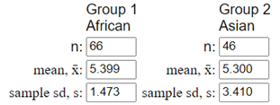
\(\mu_A\) = population mean walking distance for African elephants and \(\mu_{As}\) = population mean walking distance for Asian elephants. \(H_0: \mu_A - \mu_{As} = 0\) (no difference), \(H_a: \mu_A - \mu_{As} \neq 0\) (there is a difference). Test statistic: \(t = 0.13\text{,}\) p-value = 0.897. The standardized statistic of 0.13 indicates the observed difference is only 0.13 standard errors from 0, which is very small. The p-value of 0.897 means if there were no difference in population mean walking distances, we would observe a difference at least as extreme as ours in about 90% of random samples. We fail to reject the null hypothesis; there is insufficient evidence of a difference in mean walking distances.

3. Confidence Interval.

Also approximate a 95% confidence interval and interpret this interval in context.
Hint.
When interpreting a confidence interval for the difference, you should always clarify the direction of subtraction and which population parameter is larger. Use technology to calculate the confidence interval and remember to interpret in context.
Solution.
A 95% confidence interval for \(\mu_A - \mu_{As}\) is approximately (-1.45, 1.65) km. We are 95% confident that the true difference in mean walking distances (African minus Asian) is between -1.45 km and 1.65 km. This means African elephants could walk anywhere from 1.45 km less to 1.65 km more than Asian elephants, on average. Since this interval includes 0, it’s plausible there is no difference.

Study Conclusions.

In this study, the mean distance walked is similar for these two species (\(\bar{x}_{African} = 5.40\) vs. \(\bar{x}_{Asian} = 5.30\) km) and the sample sizes are not super large (\(n_{African}= 33\) and \(n_{Asian}= 23\)), with a fair bit of variation in walking distances within each species (\(s_{African} = 1.47\) vs. \(s_{Asian} = 3.41\) km). For these reasons, we do not expect a small p-value. The distributions are fairly symmetric so the unpooled \(t\)-test should be valid (the standard deviations are not very similar, so we would not feel comfortable assuming equal population variances). The unpooled \(t\)-test statistic of 0.131 is small, yielding a two-sided p-value of 0.897. We fail to reject the null hypothesis that the population mean walking distances are the same. These data do not provide convincing evidence of a difference in walking distances, on average, between Asian and African elephants in American zoos. A 95% confidence interval tells us that its plausible that, in these two populations, African elephants average up to 1.45 km less to 1.65 km more than Asian elephants. It might be interesting to further explore the larger variation in walking distances among the Asian elephants. We should also be aware that we have sampled a large fraction of the populations and should consider some “finite population corrections” which would only further increase the standard deviation.
Keep in mind that the \(t\)-tests only tell us about whether the centers of the distributions are significantly different. They don’t help us analyze other potentially interesting differences in the two distributions.

Subsection 19.1.4 Practice Problem 4.2A

Checkpoint 19.1.1. Verify Bootstrap Sample.

Include a screen capture of your bootstrap sample and verify you have selected 23 Asian elephants and 33 African elephants.

Checkpoint 19.1.2. Identify Multiple Selections.

Identify any elephants that were selected more than once, and explain how you can tell, AND how you can tell that the two groups were not pooled together before sampling.

Checkpoint 19.1.3. Generate Pooled Sample.

Now check the Pooled box and press Bootstrap Samples. Include a screen capture of your bootstrap sample.

Checkpoint 19.1.4. Analyze Pooled Sample.

Identify any elephants that were selected more than once, and explain how you can tell, AND how you can tell that the two groups were pooled together before sampling. (Feel free to generate a different sample if another one would make your point better.)

Checkpoint 19.1.5. Compare Simulation Methods.

Which simulation should we use for a test of significance, and which for a confidence interval? Briefly explain why.

Subsection 19.1.5 Practice Problem 4.2B

Checkpoint 19.1.6. Simulate Difference in Medians.

Use the Two sample bootstrapping applet (see also Exploration 2.9) to simulate a null distribution for the difference in medians. Do you think a t-approximation would be valid for this statistic? Why or why not.

Checkpoint 19.1.7. Compare p-values.

Approximate a p-value. Is your conclusion similar as in the analysis with means?

Checkpoint 19.1.8. Interpret Results.

Has your analysis proven that there is no difference in the median walking distances between these two species? Explain.

Subsection 19.1.6 Practice Problem 4.2C

Suppose our data had been:
Alternative elephant data scenario for Practice Problem 4.2C

Checkpoint 19.1.9. Conjecture Impact.

Conjecture how this will impact the p-value and confidence interval. Explain your reasoning.

Checkpoint 19.1.10. Verify with Technology.

Checkpoint 19.1.11. Evaluate t-procedure Validity.

Do you consider the t-procedures more valid here than for the actual study? Explain.
You have attempted of activities on this page.