Investigation 4.10: Comparison Shopping

Section 21.3 Investigation 4.10: Comparison Shopping

In this investigation, you will apply methods for paired designs to analyze data from a study comparing prices at two local grocery stores.

🔗

Exercises 21.3.1 Exercises

A student group at Cal Poly carried out a study to compare the prices at two different local grocery stores. The inventory list for Scolari’s (a privately-owned local store) was broken into 32 sheets, each with 30 items. A number between 01 and 30 was randomly generated, 17, and the 17th item on each sheet was selected.

🔗

Each student was then responsible for obtaining the price of that item at both Scolari’s and Lucky’s (which advertises itself as a discount grocery store). If the exact item was not available at both stores, the item was adjusted slightly (size or brand name) so that the identical item could be priced at both stores. Students gathered two prices for the 29 items that were found at both stores (two were found at Lucky’s but not Scolari’s). The data are available in shoppingData.txt.

🔗

1. Identify Study Components.

Identify the observational units, response variable, population, and sample in this study. Which store do you suspect will have lower prices?

Observational units:

Response variable:

Population:

Sample:

Initial conjecture:

Solution.

Obs units: grocery items
🔗

🔗
Response variable: What is the item’s price or more specifically, what is the difference in the item’s price at Lucky’s versus Scolari’s?
🔗

🔗
Population: all products common to Scolari’s and Lucky’s
🔗

🔗
Sample: 29 items
🔗

🔗
Initial conjecture: Lucky’s will have a lower average price
🔗

🔗

🔗

2. Study Design and Sampling Method.

Was this an experimental study or an observational study? Was this a simple random sample? Was it a probability sample? What is the advantage of this procedure over a simple random sample? Are there any disadvantages in selecting the sample this way?

🔗

Solution.

This was an observational study. This was not a SRS, but was a systematic sample. Advantage - very convenient and uses random selection; disadvantage - still have to find items.

🔗

3. Independent or Paired Design.

Did these students use independent samples or a paired design to collect their data?

🔗

Independent samples
Consider whether the same items are being compared at both stores.
Paired design
Correct! The same items are measured at both stores, creating natural pairs.

🔗

4. Parameter and Hypotheses.

Define the parameter of interest and state the null and alternative hypotheses corresponding to your initial conjecture.

🔗

Solution.

Let $\mu_d$ = average price difference (Lucky’s - Scolari’s)

🔗

\begin{gather*} H_0: \mu_d = 0 \text{ (no price difference on average for all the products common to both stores)}\\ H_a: \mu_d > 0 \text{ (Lucky's tends to have lower prices than Scolari's, on average)} \end{gather*}

🔗

Descriptive statistics for the items’ prices (in dollars) at each store, and for the differences in prices, as well as dotplots of the 3 distributions.

🔗

Descriptive statistics for Lucky’s prices

Descriptive statistics for Scolari’s prices

Descriptive statistics for price differences

After further investigation on the outliers among the differences, only the milk was found to be recorded incorrectly, two different sizes, and it was removed from the data set.

🔗

5. Effectiveness of Pairing.

Does the pairing appear to have been useful here? Discuss both why you suspect pairing will be beneficial in this context and any evidence in the above output.

🔗

Solution.

Yes, there is much less variability in the differences than in the prices themselves (we are comparing very different types of products with a wide range of prices).

🔗

6. Validity of Paired t-test.

Would applying a paired t-test appear to be appropriate for these data? Explain.

🔗

Solution.

Yes, the distribution of the differences is not heavily skewed, nor are there huge outliers, and our sample size is close to 30. Note, the distributions of the prices themselves are skewed to the right, but that doesn’t concern us here as we focus on the distribution of the differences.

🔗

Below is the output from R of a one-sided paired t-test and a 95% confidence interval (with milk removed):

🔗

with(shoppingData, t.test(Luckys, Scolaris, paired = TRUE, alternative="less"))
t = -1.7435, df = 27, p-value = 0.04631
alternative hypothesis: true difference in means is less than 0 
sample estimates:
mean of the differences              -0.1182
95 percent confidence interval: -0.2573 0.0209

7. Interpret Results.

What conclusions can you draw from this output? Be sure to address significance, causation, generalizability, and confidence.

🔗

Solution.

p-value = 0.046, so we have strong evidence (at 5% level) that the average price difference is positive. That is, on average, Scolari’s is more expensive per item. I’m 95% confident I will save 0.02 cents to $0.60 per item on average. Can generalize to all items at the two stores because systematic sampling used. But cannot draw a cause-and-effect conclusion as this is an observational study.

🔗

8. Prediction Interval.

Calculate (by hand) a 90% prediction interval (Investigation 2.6) based on this sample. Include a one-sentence summary of what this interval says.

🔗

Solution.

Using the $n = 28$ data set (with milk removed):

🔗

$\bar{x} = -\$0.1182\text{,}$ $s = \$0.3588$

🔗

$t^*$ with $n - 1 = 27$ degrees of freedom, 90% confidence = 1.703

🔗

$-0.1182 + 1.730(0.3588) \cdot \sqrt{1 + \frac{1}{28}} = -0.1182 + 0.622$

🔗

90% prediction interval: $(-0.74, 0.50)$

🔗

I’m 90% confident that an individual item will be anywhere from 74 cents more expensive at Scolari’s to 50 cents more expensive at Lucky’s. (Meaning, this should work -- successfully predict a price difference -- 90% of the time. So we can say roughly 90% of products have a price difference in this interval, at least with 90% confidence.)

🔗

9. Compare Interval Widths.

How does the width of this prediction interval in Question 8 compare to the width of the confidence interval for the population mean price difference in Question 7? Explain why this makes sense.

🔗

Hint.

Which is harder to predict, the mean or the next observation?

🔗

Solution.

The prediction interval is much wider than the confidence interval (but has the same midpoint). This reflects that it is harder to predict the outcome of the next observation than the average outcome of all the observations.

🔗

10. Comparing Intervals.

Which interval, the prediction interval or the confidence interval, do you find more useful here? Explain.

🔗

Solution.

It’s important to realize that they tell us different things. Do you want to know the price difference averaged across the population (e.g., to help you figure out the total bill between the two stores on all items) or do you want to know how much the price different might be on an individual item?

🔗

Note: About 6 of the 28 items (21%) are inside the confidence interval. This proportion is not supposed to be close to 0.90 because the confidence interval provides an estimate of the population mean, not individual prices. With the prediction interval 25 of 28 items (89%) are inside the prediction interval.

🔗

Study Conclusions.

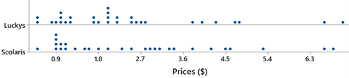
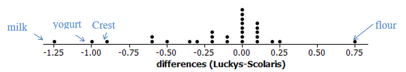
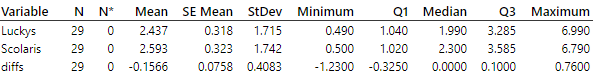
An important first step in data analysis is always to explore your data! With these data, we found some unusual observations and upon further investigation realized that one data value had been recorded in error (e.g., milk). In this case, we would be justified in removing this observation from the data file (we did not have any justification for removing the other outliers). After cleaning the data, we found that the price differences were slightly skewed to the left with a few outliers (flour, toothpaste, and frozen yogurt). The average price difference (Lucky’s $-$ Scolari’s) was $-\$0.118\text{,}$ with a standard deviation of $\$0.359\text{.}$ The median price difference was $\$0\text{.}$ So though the sample did not show a strong tendency for one store to have lower prices, the sample mean difference was in the conjectured direction. A one-sided paired t-test found that the mean price difference between these two stores was significantly less than 0 (t-value = $-1.74\text{,}$ p-value = 0.046) at the 10% level of significance, and even (barely) at the 5% level. A 95% confidence interval contained zero (as the two-sided p-value would be larger than 0.05). A 90% confidence interval for the mean price difference was ($-0.234\text{,}$ $-0.003$). We can be 90% confident that, on average, items at Scolari’s cost between 0.3 cents and 23 cents more than items at Lucky’s. This seems like a small savings but could become practically significant for a very large shopping trip. (Note, the average savings is not the same as the savings we would expect on an individual item.) In fact, we are 90% confident that an individual item will be anywhere from 74 cents more expensive at Scolari’s to 50 cents more expensive at Lucky’s. We feel comfortable generalizing these conclusions to the population of all products common to the two stores because the data were randomly selected using a probability method (systematic random sampling).

🔗

Subsection 21.3.2 Practice Problem 4.10A

For the shopping study:

🔗

Checkpoint 21.3.1. Conflicting Conclusions.

Why do the confidence interval and p-value give "conflicting" conclusions for these data?

🔗

Checkpoint 21.3.2. Predict Impact of Outlier.

Predict how the analysis will change if we don’t remove milk from the data set.

🔗

Checkpoint 21.3.3. Analysis With Milk.

Carry out a paired t-test on the 29 observations (with milk). What do you learn?

🔗

Checkpoint 21.3.4. Which Analysis to Present.

Which analysis (with or without milk) would you present to a customer? Explain.

🔗

Subsection 21.3.3 Practice Problem 4.10B

If you feel the t-procedures are not likely to be valid, another approach is a sign test (e.g., Investigation 2.7, Example 2.2).

🔗

Checkpoint 21.3.5. Sign Test Alternative.

Remove all products that have zero price difference (the ties) and count how many products are more expensive at Scolari’s vs. Lucky’s. Is this significantly more than half? You can use a binomial test or one proportion z-test (if valid) to decide and/or a confidence interval to estimate the probability a product is more expensive at Scolari’s (for all the products that do have a price difference).

🔗

Subsection 21.3.4 Practice Problem 4.10C

Checkpoint 21.3.6. Kroger vs. Food Lion Analysis.

A more recent data set was collected comparing 36 items at Kroger and Food Lion in Salem, VA over the internet during summer, 2021 ( shopping2021.txt). Food Lion advertises that it is less expensive than Kroger in general. Do you agree? Write a paragraph describing your analysis steps and conclusions.

🔗

Subsection 21.3.5 Practice Problem 4.10D

Reconsider the hippocampus values from Practice Problem 4.9B ( hippocampus.txt).

🔗

Checkpoint 21.3.7. Prediction Interval for Hippocampus Data.

Calculate and interpret a 95% prediction interval using these data.

🔗

Checkpoint 21.3.8. Validity of Procedure.

Do you believe this is a valid procedure for these data? Explain.

🔗

You have attempted of activities on this page.

🔗

Prev Top Next