Example 1.2: Cola Discrimination

Section 6.2 Example 1.2: Cola Discrimination

Try these questions yourself before viewing the solutions.

A teacher doubted whether his students could distinguish between the tastes of different brands of cola, so he presented each of his 21 students with three cups. Two cups contained one brand of cola, and the third cup contained a different brand. Which cup contained which brand was randomly determined for each student. Each student was asked to identify which cup contained the cola that was different from the other two. It turned out that 12 of the students successfully identified the "odd" cola.

🔗

Datasets and Applets page

Checkpoint 6.2.1. Test of significance.

Does this result provide strong evidence that these students do better than guessing in discriminating among the colas? Address this question with an appropriate test of significance, including a statement of the hypotheses and a p-value calculation or estimation. Be sure to clarify which procedure you used to determine the p-value and why. Summarize your conclusion, and explain the reasoning process by which it follows.

🔗

Solution.

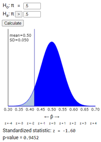
We can define \(\pi\) to be the probability that these students correctly identify the odd soda. (In other words, if this group of students were to repeat this process under identical conditions indefinitely, \(\pi\) represents the long-term fraction that they would identify correctly.) The null hypothesis asserts that the students are just guessing, which means that their success probability is one-third (\(H_0: \pi = 1/3\)). The alternative hypothesis is that students do better than guessing, which means that their success probability is greater than one-third (\(H_a: \pi > 1/3\)).

🔗

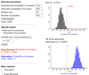
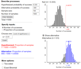
Under the null hypothesis that the students are just guessing among the three cups, \(X\) (the number of correct identifications) has a binomial distribution with parameters \(n = 21\) and \(\pi = 1/3\text{.}\) The normal distribution would probably not be valid here as we do not satisfy the conditions: \(n \times \pi = 21(1/3) = 7 < 10\text{.}\) We could simulate observations from this Binomial process using the One Proportion Inference applet, and see how often we observe 12 or more correct identifications just by chance:

🔗

R Output.

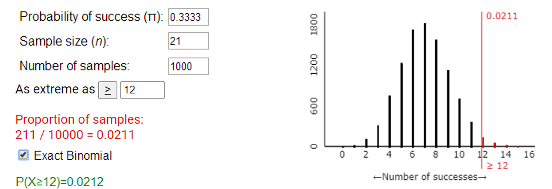
Or we could calculate the exact Binomial probability using R:

🔗

iscambinomprob(k=12, n=21, prob=.3333, lower.tail=FALSE)
# Probability 12 and above = 0.02117713

iscambinomtest(observed=12, n=21, hyp=.3333, alternative="greater")
# p-value: 0.021177

🔗

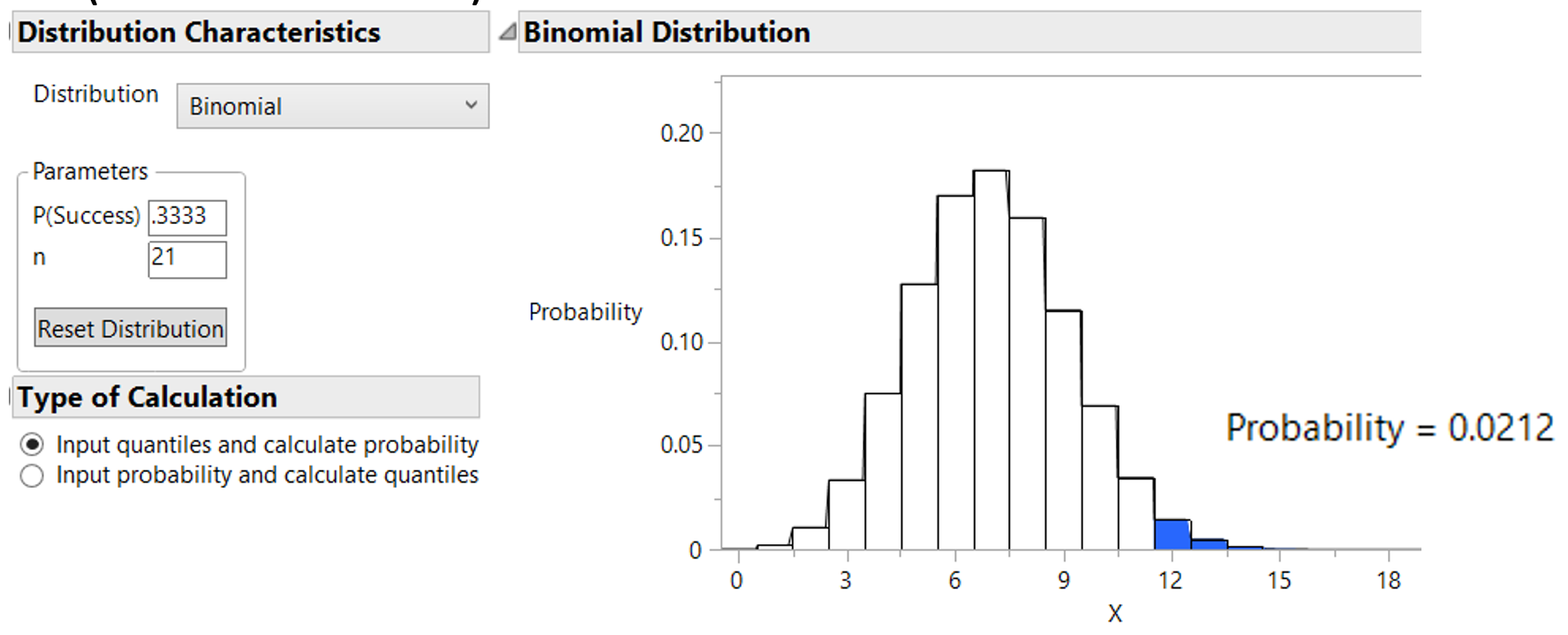
JMP Output.

Or we could calculate the exact Binomial probability using JMP:

🔗

🔗

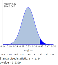
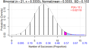
Notice the normal approximation (using R) does not provide a great estimate of this p-value:

🔗

iscamonepropztest(observed=12, n=21, hyp=.3333, alternative="greater")
# z-statistic: 2.31, p-value: 0.01031

But the normal approximation does improve with the continuity correction:

🔗

iscambinomnorm(k=12, n=21, prob=.3333, direction="above")
# binomial: 0.02118
# normal approx: 0.01031
# normal approx with continuity: 0.01860

Comparison of binomial, normal approximation, and continuity correction

This p-value reveals that if the students were just guessing, there’s only about a 2% probability of "by chance" getting 12 or more correct identifications among 21 trials. In other words, if we repeated this study over and over, and if students were just guessing each time, then a result at least this favorable would occur in only about 2% of the studies. Because this probability is quite small, we have fairly strong evidence that these students’ process in fact is better than guessing in discriminating among the colas (i.e., that \(\pi > 1/3\)). Because the sodas were randomly placed in the cups and (presumably) the teacher kept other variables (e.g., temperature, age) constant, this study attempted to isolate the taste and appearance of the sodas as the sole reasons for their selection.

🔗

Checkpoint 6.2.2. Calculate confidence interval.

Calculate a 95% confidence interval based on these sample data. Clearly define the parameter that this interval estimates, and interpret the interval.

🔗

Solution.

If we calculate the default binomial interval we find (e.g., in R):

🔗

iscambinomtest(12, 21, conf.level=95)
# 95% Confidence interval for pi: (0.34021, 0.7818)

So we are 95% confident that the underlying probability of a correct identification for these students is between 0.340 and 0.782.

🔗

Checkpoint 6.2.3. Apply significance level.

Would this teacher be convinced that his students do better than guessing if he uses the 0.05 significance level?

🔗

Solution.

Yes, the p-value is less than 0.05, so with that significance level, the teacher would be convinced that his students do better than guessing in discriminating among the colas. Notice also that 1/3 is not captured in the 95% confidence interval.

🔗

Checkpoint 6.2.4. Identify Type I and Type II errors.

Describe what Type I and Type II errors mean in this situation. Which type of error might you have made in Checkpoint 6.2.3?

🔗

Solution.

A Type I error would mean that these students are actually just guessing, but we erroneously conclude that they do better than guessing. A Type II error would mean that the students are not just guessing, but we do not consider the evidence strong enough to conclude that. With this small p-value we might have made a Type I error, but it would be impossible for us to have made a Type II error.

🔗

Checkpoint 6.2.5. Check normal approximation validity.

Suppose the students want to redo the study with 100 students. Would a normal approximation be valid in this case? Justify your answer.

🔗

Solution.

Now the normal approximation should be valid. If we assume \(\pi = 1/3\text{,}\) then \(n\pi = 100(1/3) \approx 33.3 > 10\) and \(n(1-\pi) = 100(2/3) \approx 66.7 > 10\text{.}\) (If \(\pi\) is larger than 1/3 as we suggested above, this approximation is even more valid.)

🔗

Checkpoint 6.2.6. Calculate power of test.

Using the 0.05 significance level and a sample size of 100 students, calculate the power of the test when the underlying probability equals 0.5, and interpret your result.

🔗

[Hint: Remember our two-step process: 1) Find the rejection region under the null hypothesis, now using the normal distribution; 2) Determine the probability of being in the rejection region under an alternative value of the parameter.]

🔗

Solution.

If we want to test \(H_0: \pi = 1/3\) vs. \(H_a: \pi > 1/3\) for a sample size of \(n = 100\text{,}\) then the rejection region will be the values of \(\hat{p}\) so that \(P(\hat{p} > \text{cut-off}) \leq 0.05\) when \(\pi = 1/3\text{.}\) Because we are comfortable using the normal approximation with this sample size, we can use the Theory-Based Inference applet to find this cut-off.

🔗

(Enter the hypothesized value, the direction of the alternative, the sample size, then change the count input until the p-value dips below 0.05). This says a \(\hat{p}\) of 0.420 or larger would lead us to reject this null hypothesis that \(\pi = 0.5\) at the 5% level of significance.

🔗

So now we need to find the probability \(P(\hat{p} \geq 0.420)\) when the underlying process probability is actually 0.5. When \(\pi = 0.5\text{,}\) we have an approximately normal distribution with mean equal to 0.5 and standard deviation equal to \(\sqrt{.5(.5)/100} = 0.05\text{.}\) Using the Theory-Based Inference applet, we can enter 0.5 as the hypothesized probability and 0.420 as the observed sample proportion with a > alternative. This gives us an appropriate power of 0.9452.

🔗

Thus, the probability of rejecting \(H_0: \pi = 1/3\) when \(n = 100\) and \(\pi\) is actually 0.5 equals 0.9452. Therefore, in about 95% of samples from a process with \(\pi = 0.5\) we will correctly reject that \(\pi = 1/3\text{.}\)

🔗

Showing these curves on the same graph:

🔗

🔗

Checkpoint 6.2.7. Power with larger probability.

If the underlying probability of identifying the odd soda equals 2/3, will the power calculated in Checkpoint 6.2.6 be larger or smaller in this case? Explain without performing any calculations.

🔗

Solution.

If the underlying process probability is even larger at \(\pi = 2/3\text{,}\) this will shift the alternative distribution to the right and even more of the distribution will lie in the rejection region. Our power will increase as it will be even easier for us to obtain a sample that will convince us that the hypothesized value of 1/3 is incorrect.

🔗

🔗

Checkpoint 6.2.8. Power with stricter significance level.

If the teacher uses a 0.01 significance level (with an alternative probability of 0.50), will the power calculated in Checkpoint 6.2.6 be larger or smaller in this case? Explain without performing any calculations.

🔗

Solution.

If the level of significance is lowered from 0.05 to 0.01, this will move the red line to the right. We will need a larger sample proportion to convince us and this will slightly reduce our power (less than 0.90).

🔗

🔗

Watch video walkthrough of this example.

🔗

You have attempted of activities on this page.

🔗

Prev Top Next