Investigation 1.4: Heart Transplant Mortality

Section 3.4 Investigation 1.4: Heart Transplant Mortality

In this investigation, you will explore what factors of a study impact the magnitude of the p-value.

Exercises 3.4.1 The Study

Poloneicki, Sismanidis, Bland, and Jones (2004) reported that in September 2000 heart transplantation at St. George’s Hospital in London was suspended because of concern that more patients were dying than previously. Newspapers reported that the 80% mortality rate in the last 10 cases was of particular concern because it was over five times the national average. The variable measured was whether or not the patient died within 30 days of the transplant. Although there was not an officially reported national mortality rate (probability of death within 30 days for patients undergoing this procedure), the researchers determined that 15% was a reasonable benchmark for comparison.

🔗

1. Define Sample and Variable.

Define the sample or random process for this study.

🔗

Hint.

Think about what is being observed repeatedly.

🔗

Solution.

The 10 most recent heart transplantation surgeries at St. George’s Hospital (or more generally, heart transplantation surgeries at this hospital, across all the patients)

🔗

2. Define the Variable.

Define the variable for this study.

🔗

Hint.

What outcome is being measured for each observation?

🔗

Solution.

Whether or not the patient died within 30 days of the transplant

🔗

Note: We define "success" as death within 30 days (could be either death or survival, but this matches the 15% parameter), and "failure" as survival.

🔗

3. Variable Type.

Is this variable quantitative or categorical?

🔗

Quantitative
Not quite. This variable has categories (death or survival), not numerical measurements.
Categorical
Correct! This is a categorical variable with two categories (binary): death within 30 days or survival.

Solution.

Categorical (binary)

🔗

We need to consider which outcome we will consider "success" and which we will consider "failure." The choice is often arbitrary, though sometimes we may want to focus on the more unusual outcome as success. In fact, in many epidemiology studies, "death" is typically the outcome of interest or "success."

🔗

4. Define Parameter.

Considering death within 30 days as a success, define the parameter of interest in this study (in words).

🔗

Hint.

What long-run proportion or probability are we interested in?

🔗

Solution.

Parameter: The underlying probability of death within 30 days of transplant at this hospital.

🔗

5. Parameter Symbol.

What symbol should we use to represent this parameter?

🔗

Hint.

Look for the Greek letter used for a process probability in a binomial distribution.

🔗

\(\hat{p}\)
This is the symbol for the sample proportion (statistic), not the population parameter.
\(\pi\)
Correct! We use \(\pi\) to represent the probability of success in a binomial process.
\(\mu\)
This is the symbol for a population mean, not a probability.
\(p\)
While p is sometimes used for probability, we use the Greek letter \(\pi\) for the process probability parameter.

Solution.

We use \(\pi\) to represent the probability of death within 30 days.

🔗

6. Is this a Binomial Process?

Is it reasonable to model this heart transplantation process as a binomial process?

🔗

Hint.

Check the four conditions for a binomial process: two outcomes, fixed number of trials, independence, and constant probability.

🔗

Solution.

Yes, this is a binomial process if we assume the transplants are independent and the probability of death is the same for each transplant patient.

🔗

7. Nothing Unusual Hypothesis.

If there is nothing unusual about the mortality rate for heart transplantations at this hospital (compared to other U.K. hospitals), what does this imply about the value of the probability of "success"?

🔗

\(\pi\)

🔗

Hint.

What was stated as the reasonable benchmark for comparison?

🔗

Solution.

\(\pi = 0.15\)

🔗

8. Higher Rate Hypothesis.

If the patients at this hospital are indeed dying at a higher rate than the benchmark rate, what does this imply about the value of the probability of "success"?

🔗

Hint.

If the rate is higher than 15%, what inequality would describe \(\pi\text{?}\)

🔗

\(\pi\)

🔗

Solution.

\(\pi > 0.15\)

🔗

9. State Hypotheses.

Translate your answers to the previous questions to null and alternative hypothesis statements. Keep in mind, the null hypothesis claims the observed result is "just by chance," whereas the alternative hypothesis translates the research conjecture.

🔗

Match each hypothesis type with the correct statement:

🔗

Hint.

The null hypothesis typically states equality, while the alternative states the direction of the research suspicion.

🔗

Alternative Hypothesis (\(H_a\))
\(\pi\) > 0.15 (the death rate at St. George’s is larger than the national average)
Null Hypothesis (\(H_0\))
\(\pi\) = 0.15 (the death rate at St. George’s is the same as the national average)

🔗

10. Direction of Sample Result.

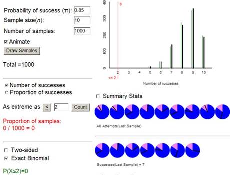
Of the hospital’s ten most recent transplantations at the time of the study, there had been eight deaths within the first 30 days following surgery. Is this sample result in the direction suspected by the researchers? Explain.

🔗

Hint.

Compare 8/10 = 0.80 to the benchmark of 0.15.

🔗

Solution.

\(\hat{p} = 8/10 = 0.8\)

🔗

Because 0.8 > 0.15, yes, the result is in the conjectured direction.

🔗

Technology Detour – Calculating Binomial Probabilities.

You could use the One Proportion Inference applet to use simulation or the binomial distribution to find the p-value. Many statistical software packages will carry out a "Binomial test" directly.

🔗

11. Binomial Test of Significance.

Use R or JMP to find and report the p-value for the Heart Transplant study (8 deaths in 10 trials with hypothesized probability 0.15). Choose one set of instructions below by clicking on a hint. Report the p-value you find.

🔗

p-value:

🔗

Hint 1. R Instructions

The iscambinomtest function takes the following inputs:

🔗

observed = Observed number of successes or proportion of successes
🔗

🔗
n = Number of trials (sample size)
🔗

🔗
hypothesized = Hypothesized probability
🔗

🔗
alternative = Direction of alternative (e.g., "greater" or "less" or "two.sided")
🔗

🔗

The following code finds the p-value for the infant study study:

🔗

You should see the p-value in the output as well as a graph of the binomial distribution with the upper tail shaded. Modify the code for the heart transplant study, in particular, what are you setting the hypothesis value to?

🔗

R Reminder: The alternative parameter controls the direction: "greater" tests if \(π > 0.5\text{,}\) "less" tests if \(π < 0.5\text{.}\)

🔗

Hint 2. JMP Instructions

Using the Distribution Calculator in the ISCAM Journal File (Download this file to your computer and then open the .jrn file to launch JMP.)

🔗

Choose Analyze > Distribution
🔗
- With raw data, drag the variable to the Y, Columns slot. Press OK.
  🔗
  
  🔗
- With summarized data, move the column with the category names to the Y, columns slot and move the column with the counts to the Freq slot. Press OK.
  🔗
  
  🔗
🔗

JMP Test Probabilities dialog showing setup for binomial test

From the variable’s hot spot, select Test Probabilities.
🔗

🔗
Specify the hypothesized probability of success for the category you want to define as success (only).
🔗

🔗
Then pick a one-sided alternative hypothesis (greater than or less than).
🔗

🔗
Press Done.
🔗

🔗

JMP output showing binomial test results with p-value

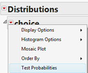
JMP assumes "success" to be the first category alphabetically unless you specify otherwise with Cols > Column Info > Column Properties > Value Ordering.

🔗

Note: "Not equal to" alternatives will be discussed in Investigation 1.5.

🔗

Solution.

For the Heart Transplant study with 8 deaths out of 10 trials and a hypothesized probability of 0.15:

🔗

p-value = P(X ≥ 8) = 0.00000866 (or 8.665 × 10\(^{-6}\))

🔗

This extremely small p-value provides very strong evidence that the death rate at this hospital exceeds the national benchmark of 0.15.

🔗

12. Interpret the p-value.

Provide a detailed interpretation of your p-value:

🔗

The p-value is the probability of obtaining or successes in trials from a random process, assuming .

🔗

Hint.

Fill in the blanks with the specific numbers and assumption from this context.

🔗

Solution.

This is the probability of getting 8 or more "successes" out of 10 observations from a random process where the long-run probability of success equals 0.15.

🔗

13. Draw Conclusions.

Evaluate your p-value: what conclusions would you draw about the probability of death within 30 days of a heart transplant at this hospital?

🔗

Hint.

Consider how small the p-value is and what that suggests about the null hypothesis.

🔗

Solution.

We have very strong evidence in favor of \(\pi > 0.15\) (\(H_a\)). We don’t think the higher mortality rate observed in these 10 cases happened just by chance.

🔗

Does it matter which outcome I choose to be success?

Suppose that we had focused on survival for 30 days rather than death within 30 days as a "success" in this study.

🔗

14. Alternative Success Definition.

Describe how the hypotheses would change and how the calculation of the binomial p-value would change. Then go ahead and calculate and interpret the exact binomial p-value with this set-up. How does its value compare to your answer in the previous question? How (if at all) does your conclusion change?

🔗

Hint.

If survival is success, then the benchmark becomes 0.85. How many survived out of 10?

🔗

Hint 1. R option

🔗

Hint 2. One Proportion Inference applet

🔗

Solution.

The null hypothesis would be \(H_0: \pi = 0.85\) and the alternative hypothesis would be \(H_a: \pi < 0.85\text{.}\)

🔗

Binomial distribution showing survival as success with pi=0.85

This turns out to be an equivalent analysis.

🔗

15. Compare p-values.

Compared to the analysis with death as success, the p-value has:

🔗

Hint.

Compare the p-value from the death analysis to the survival analysis.

🔗

Increased
Stayed the same
Decreased

🔗

16. Impact on Conclusion.

Compared to the analysis with death as success, does the conclusion change when we use survival as success?

🔗

Hint.

Does changing the definition of success affect the strength of evidence?

🔗

No change - the conclusion remains the same
Yes - it is no longer significant
Yes - it is now significant

🔗

Does the sample size matter?

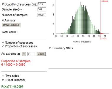
Following up on the suspicion that the sample of size 10 aroused, these researchers proceeded to gather data on the previous 361 patients who received a heart transplant at this hospital dating back to 1986. They found 71 deaths within 30 days among heart transplantations.

🔗

17. Calculate Sample Proportion.

Calculate the sample proportion of deaths for these data:

🔗

Hint.

Sample proportion = 71/361.

🔗

Solution.

\(\hat{p} = 71/361 = 0.197\)

🔗

18. Predict Strength of Evidence.

Predict whether this is more or less convincing evidence that this hospital’s death rate exceeds 0.15. Explain your reasoning.

🔗

Hint.

Compare the sample proportion (0.197) to 0.15. Also consider that with a larger sample size, we have more information.

🔗

Solution.

This sample proportion is much closer to 0.15 but also based on a much larger sample size. Predictions will vary by student.

🔗

19. Calculate p-value with Technology.

Use technology to determine the binomial probability of finding at least 71 deaths in a sample of 361 if \(\pi = 0.15\text{.}\)

🔗

p-value:

🔗

Hint 1.

Use the One Proportion Inference applet or R or JMP with n=361, observed=71, and π=0.15, with "greater than"

🔗

Hint 2. R option

🔗

Hint 3. One Proportion Inference applet

🔗

Solution.

Binomial distribution for n=361 with pi=0.15 showing p-value

p-value ≈ 0.01

🔗

20. Evaluate Larger Sample Evidence.

Is the probability you found convincing evidence to consider the sample result surprising if the mortality rate at this hospital matched the national rate? Explain.

🔗

Hint.

Consider how small the p-value is - what threshold are you using?

🔗

Solution.

Yes, small p-value. Reject \(H_0\) that \(\pi = 0.15\text{,}\) convinced that \(\pi > 0.15\text{.}\)

🔗

21. Compare Strength of Evidence.

Is the evidence against the null hypothesis stronger or weaker than the earlier analysis based on 10 deaths? Explain how you are deciding and why the strength of evidence has changed in this manner.

🔗

Hint.

Compare the two p-values. Which is smaller?

🔗

Solution.

The evidence is a bit weaker (though still quite strong) demonstrated by the larger p-value.

🔗

22. Expected Number of Deaths.

Calculate the expected number of deaths, E(X), for each sample size.

🔗

\(n = 10: E(X) =\)

🔗

\(n = 361: E(X) = \)

🔗

Hint.

Use the formula \(E(X) = n \times\pi\) where \(\pi = 0.15\text{.}\)

🔗

Solution.

\(E(X)\) = 10(0.15) = 1.5 or 361(0.15) = 54.15

🔗

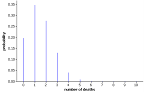
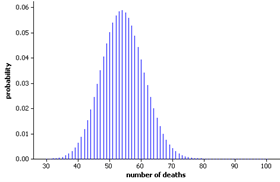
The following graphs display the two theoretical probability distributions (for sample sizes \(n = 10\) and \(n = 361\)), both assuming the null hypothesis (\(\pi = 0.15\)) is true. These graphs show just how far the observed values (8 and 71) are from the expected value of the number of deaths (0.15 × 10 = 1.5 and 0.15 × 361 = 54.15) in each case. You should also note that the shape, center, and variability of the probability distribution for number of successes are all affected by the sample size \(n\text{.}\)

🔗

Binomial distributions for n = 10 and n = 361, both with π = 0.15

🔗

Binomial distribution showing n=10, pi=0.15, with observed value of 8 marked

Binomial distribution showing n=361, pi=0.15, with observed value of 71 marked

Keep in mind that of interest to us is the observed statistic’s relative location in the null distribution. Thus, we are most interested in how variable the possible outcomes are from the "expected" outcome. The center of the distribution isn’t all that interesting to us in answering the research question because we determine what the center of the distribution will be by how we specify the null hypothesis. Even the shape isn’t all that interesting on its own in answering our research question.

🔗

23. Distribution Feature Differences.

Identify another feature (beside center, shape, and variability) of the above distributions that differs between them.

🔗

Hint.

Think about practical aspects like the scale or range of values displayed.

🔗

Solution.

The most obvious difference is how close together the spikes are.

🔗

24. Standardize Second Dataset.

How many standard deviations is the observed sample proportion above the hypothesized probability for the second dataset?

🔗

Expected value when \(n = 361\) and \(\pi = 0.15\text{:}\)

🔗

SD when \(n = 361\) and \(\pi = 0.15\text{:}\)

🔗

Number of standard deviations 71 is above the expected value:

🔗

Hint.

Use \(E(X) = n × π\) and \(SD(X) = \sqrt{n × π × (1-π)}\text{.}\) Then calculate \((71 - E(X))/SD(X)\text{.}\)

🔗

Solution.

\(SD(X) = \sqrt{361 × 0.15 × 0.85} = 6.78\)

🔗

Observed 71

🔗

\((71 - 54.15)/6.78 ≈ 2.49\text{.}\) This is larger than 2.

🔗

For first data set: \((8 - 1.5)/\sqrt{10 × 0.15 × 0.85} = 6.5/1.13 = 5.75\) (this shows us that the evidence is a fair bit stronger with the first data set)

🔗

25. Evaluate Standardized Evidence.

Does this calculation also provide strong evidence against the null hypothesis? How are you deciding?

🔗

Hint.

Consider whether being 2.49 standard deviations from the expected value is unusual.

🔗

Solution.

Yes, this provides strong evidence against the null hypothesis. A result more than 2 standard deviations from the expected value is generally considered unusual, and 2.49 SD is quite far from the mean.

🔗

26. Which Dataset is More Valid?

In your opinion, which data set do you think is more valid to use – the larger sample size or the more recent data? Explain how you are deciding.

🔗

Hint.

Consider the trade-offs: more data vs. more current/relevant data. Also think about "data snooping."

🔗

Solution.

Opinions will vary. The larger sample size is more likely to give us more precise results but some based on very old data which may no longer be representative of the current process.

🔗

Study Conclusions.

A sample mortality rate of 80% is indeed quite surprising, even with a sample size as small as 10, if the actual probability of death were 0.15. The (exact) p-value is 0.0000087, and the observed statistic is 5.76 standard deviations above the expected value, providing extremely strong evidence that the actual probability of death at this hospital is higher than the national benchmark of 0.15 (fewer than 1 in 100,000 sets of 10 operations would "randomly" have 8 or more deaths if \(\pi = 0.15\)). However, we must be cautious about doing this type of "data snooping," where we allowed a seemingly unusual observation to motivate our suspicion and then use the same data to support our suspicion. Once the initial suspicion has formed, we should collect new data on which to test the suspicion. The actual investigation examined all previous heart transplantations at this hospital over the previous 14 years. In this broader study, the p-value is 0.0097 and the observed number of successes is 2.48 standard deviations above the expected number, still providing very strong evidence against the null hypothesis. That is, there is strong evidence that this hospital’s probability of mortality was higher than the 15% national benchmark. We must, however, be cautious because our study has not identified what factors could be leading to the higher rate. Perhaps this hospital tends to see sicker patients to begin with. The researchers actually performed a more sophisticated analysis that incorporated information about the risk factors of all the operations at this hospital and reached similar conclusions.

🔗

Subsection 3.4.2 Practice Problem 1.4A

In April 2014, the city of Flint Michigan switched its water supply to the Flint River in an effort to save money. The U.S. Environmental Protection Agency (EPA)’s Lead and Copper Rule states that if lead concentrations exceed an action level of 15 parts per billion (ppb) in more than 10% of homes sampled, then actions must be undertaken to control corrosion, and the public must be informed. In the initial sample of 71 homes, 8 tested above 15 ppb.

🔗

Checkpoint 3.4.1. Binomial Process Justification.

Suppose our variable is "was the lead concentration level above 15 ppb?". Is it reasonable to model this as a binomial process? Justify your response for each condition. Be sure to explain how you are defining success and any assumptions you are making about the process.

🔗

Checkpoint 3.4.2. Define Parameter.

Define (in words) the parameter of interest.

🔗

Checkpoint 3.4.3. State Hypotheses.

State null and alternative hypotheses for testing whether the probability of a house testing above 15 ppb is more than 0.10.

🔗

Checkpoint 3.4.4. Calculate p-value.

Report the binomial p-value for your hypotheses.

🔗

Checkpoint 3.4.5. Modified Dataset p-value.

After dropping two "suspicious" observations, 6 of the 69 remaining observations were above 15 ppb. Report the binomial p-value for your hypotheses. Is the second p-value larger or smaller than the first?

🔗

Subsection 3.4.3 Practice Problem 1.4B

Reconsider the wolf (Yukon) who correctly understood a communicative cue in 7 of 8 attempts. Let \(\pi\) represent the probability of Yukon identifying the correct container with a communicative cue.

🔗

Checkpoint 3.4.6. Greater Than Alternative.

If the alternative hypothesis is \(H_a: \pi > 0.50\text{,}\) what is the p-value? Based on this p-value, state an appropriate conclusion in terms of the alternative hypothesis.

🔗

Checkpoint 3.4.7. Less Than Alternative.

If the alternative hypothesis is \(H_a: \pi < 0.50\text{,}\) what is the p-value? Based on this p-value, state an appropriate conclusion in terms of the alternative hypothesis.

🔗

Checkpoint 3.4.8. When p-value Exceeds 0.50.

Under what circumstances will a p-value calculation like these be larger than 0.50?

🔗

Subsection 3.4.4 Practice Problem 1.4C

One of the first times the U.S. Supreme Court considered statistical significance in an employment discrimination case was in Hazelwood School District vs. United States (1977). The U.S. government sued the City of Hazelwood, a suburb of St. Louis, MO, on the grounds that it discriminated against African Americans in its hiring of school teachers. The evidence introduced noted that of the 405 teachers hired in 1972 and 1973 (the years following the passage of the Civil Rights Act), only 15 had been African-American. By comparison, according to 1970 census figures, of the almost 20,000 elementary and secondary teachers employed in the St. Louis area, 15.4% were African American. We want to decide whether the data on these 405 teachers is convincing evidence that the Hazelwood hiring process had a probability of a new hire being African American that was less than 0.154.

🔗

Checkpoint 3.4.9. Expected Number of Hires.

What is the expected number of African-American hires in a sample of 405 teachers if the probability of a new hire being African American equals 0.154?

🔗

Checkpoint 3.4.10. Standardize and Conclude.

Using the binomial distribution, how many standard deviations is 15 from the expected number of new hires that are African American when the null hypothesis is true?

🔗

Number of standard deviations:

🔗

What conclusion would you draw?

🔗

Checkpoint 3.4.11. Excluding St. Louis City.

The St. Louis City School District had recently followed a policy attempting to maintain a 50% African-American teaching staff. If you exclude the St. Louis City School District, then the proportion of eligible teachers in the St. Louis area that were African-American was 0.057. What is the new expected number of hires? What conclusions would you draw?

🔗

Checkpoint 3.4.12. Importance of Labor Market Definition.

Discuss briefly how this case illustrates "the importance of the choice of the relevant labor market area" in cases of discrimination.

🔗

You have attempted of activities on this page.

🔗

Prev Top Next