Investigation 3.1: Teen Hearing Loss (cont.)

Section 13.1 Investigation 3.1: Teen Hearing Loss (cont.)

Exercises 13.1.1 The Study

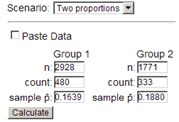
The Shargorodsky, Curhan, Curhan, and Eavey (2010) study from Investigation 1.14 actually focused on comparing the current hearing loss rate among teens (12-19 years) to previous years to see whether teen hearing loss is increasing, possibly due to heavier use of ear buds. In addition to the 1,771 participants in the NHANES 2005-6 study (333 with some level of hearing loss), they also had hearing loss data on 2,928 teens from NHANES III (1988-1994), with 480 showing some level of hearing loss. Our goal is to assess whether the difference between these two samples can be considered statistically significant.

🔗

1. Study Design Difference.

What is the primary difference between this study and those examined in ISCAM Chapters 1 and 2?

🔗

Solution.

Comparing two samples to each other

🔗

2. Identify Populations and Variable.

Identify the two populations.

🔗

Identify the variable.

🔗

Solution.

populations: (1) 2005-6 teens; (2) 88-94 teens

🔗

Variable: whether/not some hearing loss.

🔗

3. Variable Type.

Identify the variable type.

🔗

Categorical
Quantitative

Solution.

The variable is binary categorical (hearing loss: yes/no).

🔗

Descriptive Statistics.

When we have two samples for a binary categorical variable, it is often useful to organize the data using a two-way table.

🔗

4. Two-Way Table.

Complete the following 2 × 2 table of counts.

🔗

Hearing loss? \ Time frame	1988-1994	2005-2006
Some hearing loss
No hearing loss
Total	2928	1771

Solution.

	1988-1994	2005-2006	Total
Some hearing loss	480	333	813
No hearing loss	2448	1438	3886
Total	2928	1771	4699

🔗

5. Comparing Counts.

Explain why it does not make sense to conclude that hearing loss was more prevalent in 1988-1994 than in 2005-2006 based only on the comparison that 480 > 333.

🔗

Solution.

Because the sample sizes for the two surveys are not the same

🔗

6. Comparing Proportions.

Suggest a better way to compare the prevalence of hearing loss between the two studies. Calculate one number as the statistic for this study (what symbols are you using?). Does your statistic seem large enough to convince you that there has been an increase in hearing loss?

🔗

Solution.

\(\hat{p}_{88} - \hat{p}_{05}\) = 480/2928 - 333/1771 = -0.024 (judgements of the impressiveness of this number will vary; it seems on the small side but the sample sizes are large)

🔗

Definition: Conditional Proportions.

The simplest statistic for comparing a binary variable between two groups is the difference in the proportion of "successes" for each group. These proportions, calculated separately for each group rather than looking at the overall proportion, are called conditional proportions.

🔗

In this case, we compute the difference in the proportion of teens with some level of hearing loss between the two years \((\hat{p}_{94} - \hat{p}_{06} = 480/2928 - 333/1771)\text{.}\)

🔗

The next step is to examine an effective graphical summary for comparing the two groups.

🔗

Technology Detour – Segmented Bar Graphs.

Use technology to create numerical and graphical summaries for these summarized data.

🔗

Hint 1. R Instructions

Create (and view) a matrix in R to store the counts from the two-way table:

🔗

Convert to a matrix of conditional proportions (margin = 2 for column proportions):

🔗

Create a segmented bar graph:

🔗

Hint 2. JMP Instructions

You can specify the counts from the two-way table, but you have to do so in "column format" (each row is a combination of the two variables and the counts are all in one column)

🔗

Select Analyze > Fit Y by X .
🔗

🔗
Click Hearing Loss then click the Y, Response button (or drag).
🔗

🔗
Click Year then click the X, Factor button (or drag). (With raw data, you would be done here.)
🔗

🔗
Finally click Count then the Freq button. Click OK.
🔗

🔗
Right-click on one of the bars and select Cell Labelling > Show Percents.
🔗

🔗

🔗

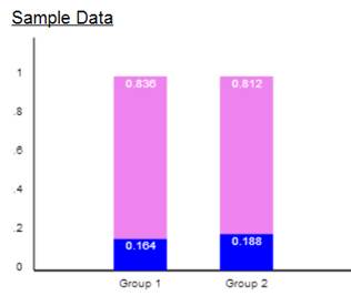
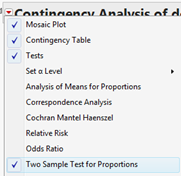
JMP creates a "Mosaic Plot" (the column widths also reflect the relative sample sizes). An extended two-way table is shown below the Mosaic Plot although the rows and columns are reversed. Click the red Contingency Table arrow and uncheck Col% and Total% to see a less cluttered table.

🔗

7. Descriptive Statistics.

Write a sentence or two comparing the distributions of hearing loss between these two studies. Be sure to report an appropriate statistic.

🔗

Solution.

A slightly higher proportion of teens (0.024) had some level of hearing loss in the 2005/6 data than in 1998-94.

🔗

8. Initial Comparison.

Do these data convince you that there is a difference in the population proportions? If not, what could be another explanation for the difference you see in these numerical and graphical summaries for these two samples?

🔗

Solution.

Judgements will vary, but we should still consider random sampling "error"

🔗

Inferential Statistics.

As we’ve said before, it certainly is possible to obtain sample proportions this far apart, just by random chance, even if the population proportions (of teens with some hearing loss) were the same. The question now is how likely such a difference would be if the population proportions were the same.

🔗

We can answer this question by modeling the sampling variability, arising from taking independent random samples from these populations, for the difference in two sample proportions. Investigating this sampling variability will help us to assess whether this particular difference in sample proportions is strong evidence that the population proportions actually differ.

🔗

Animated illustration of sampling variability in two proportions

9. Hypotheses.

Let \(\pi_{94}\) represent the proportion of all American teenagers in 1994 with at least some hearing loss, and similarly for \(\pi_{06}\text{.}\) Define the parameter of interest to be \(\pi_{94} - \pi_{06}\text{,}\) the difference in the population proportions between these two years. State appropriate null and alternative hypotheses about this parameter to reflect the researchers’ conjecture that hearing loss by teens is becoming more prevalent.

🔗

\(H_0: \)

🔗

\(H_a: \)

🔗

Solution.

\(H_0: \pi_{94} = \pi_{06}\) or \(\pi_{94} - \pi_{06} = 0\) (the population proportions are the same)

🔗

\(H_a: \pi_{94} - \pi_{06} < 0\) or \(\pi_{94} < \pi_{06}\) (a higher rate of hearing loss in 2006 than in 1994)

🔗

Success = some hearing loss

🔗

Simulation.

Because the population sizes are very large compared to the sample sizes, we will model this by treating the populations as infinite and sampling from binomial processes.

🔗

10. Modeling Null Hypothesis.

How do we model the null hypothesis being true?

🔗

Solution.

We sample from two random processes but we keep the process probability the same between them.

🔗

So under the null hypothesis we really only have one value of \(\pi\) to estimate – the common population proportion with hearing loss for these two years.

🔗

11. Pooled Estimate.

What is your best estimate for \(\pi\) from the sample data (assuming the null hypothesis is true)?

🔗

Hint.

Think about combining the two years together.

🔗

Solution.

\(\hat{\pi}\) = 813/4699 = 0.173

🔗

12. Simulation Design.

Describe how you could carry out a simulation analysis to investigate whether the observed difference in sample proportions provides strong evidence that the population proportions with hearing loss differed between these two time periods. How will you estimate the p-value?

🔗

Solution.

We could take random samples of 2928 and 1771 from two populations that have the same population proportion of successes. Then see how often 1 - 2 ≈ -0.024 when 94 - 06 = 0 by random sampling alone.

🔗

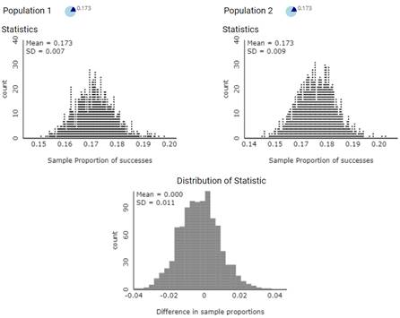
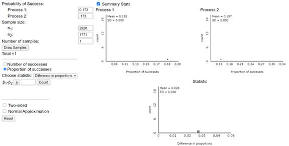
We will begin our simulation analysis by assuming the (common) population proportion is actually this value (\(\pi = 0.173\)). We simulate the drawing of two different random samples from this population, one to represent the 1994 study and the other for the 2006 study. Then we examine the distribution of the difference in the conditional proportions with some hearing loss between these two years. Finally, we repeat this random sampling process for many trials. [Note: We can assume \(\pi = 0.173\) without loss of generality, but you might want to verify this with other values for \(\pi\) as well.]

🔗

Use the Comparing Two Population Proportions applet to randomly sample one "could have been" difference in conditional proportions assuming the null hypothesis is true.

🔗

Specify .173 as the process probability for both populations.
🔗

🔗
Specify 2928 and 1771 as the two sample sizes.
🔗

🔗
Leave the Number of samples set to 1.
🔗

🔗
Press Draw Samples.
🔗

🔗

🔗

13. One Repetition.

Report the values you found for \(\hat{p}_1\text{,}\) \(\hat{p}_2\text{,}\) and \(\hat{p}_1 - \hat{p}_2\text{.}\)

🔗

Hint.

See Technology Detour below for carrying out these simulations in other software packages.

🔗

\(\hat{p}_1 = \) \(\hat{p}_2 = \) \(\hat{p}_1 - \hat{p}_2 = \)

🔗

Solution.

Example results, \(\hat{p}_1\) =0.185 and \(\hat{p}_2\) = 0.157 for a difference of 0.028.

🔗

14. Variability.

Will everyone in the class get the same answers to Question 12? Explain.

🔗

Solution.

No, because of the randomness in the sampling process not everyone will get the same answers to checkpoint 16.

🔗

To learn about the pattern of variation in our statistic, we want to generate many more outcomes assuming the null hypothesis to be true.

🔗

Change the Number of samples from 1 to 999

🔗
Press Draw Samples for a total of 1,000 independent pairs of random samples.

🔗

15. Many Repetitions.

Describe the distribution of \(\hat{p}_1\) values, the distribution of \(\hat{p}_2\) values, and the distribution of \(\hat{p}_1 - \hat{p}_2\) values. Does the distribution of difference in proportions behave as you expected? In particular, does the mean of this distribution make sense? (How does it compare to the means of the individual \(\hat{p}\) distributions?) Explain.

🔗

Solution.

Answers will vary but should expect the distributions of sample proportions (with large sample sizes) to each be approximately normal with means equal to the (same) population proportion and for the mean of the differences (assuming the null is true) to be close to zero.

🔗

Example results:

🔗

The distributions of the values should be approximately normal with means around 0.173. The standard deviations should be around 0.007 and 0.009. The distribution of the 1-2 values should be approximately normal with mean around 0 (0.173 - 0.173) and standard deviation around 0.011, which is larger than the individual distribution SDs.

🔗

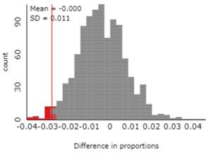
Now determine the empirical p-value by counting how often the simulated difference in conditional proportions is at least as extreme as the actual value observed in the study by entering the observed value in the Count Samples box and pressing the Count button. (Make sure the direction matches the alternative hypothesis.)

🔗

16. Empirical p-value.

Report your empirical p-value and indicate what conclusion you would draw from it.

🔗

Solution.

Example results

🔗

This is a small p-value and provides moderate evidence against the null hypothesis in favor of the alternative hypothesis that the population proportion with at least some level of hearing loss was greater in 2006 than in 1994.

🔗

Mathematical Model.

It turns out that there is no "exact" method for calculating the p-value here, because the difference in two binomial variables does not have a binomial, or any other known, probability distribution.

🔗

17. Distribution Shape.

However, did the histogram of \(\hat{p}_1 - \hat{p}_2\) values you examined remind you of any other probability distribution?

🔗

Solution.

The normal distribution

🔗

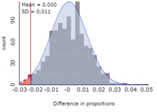
Check the Normal Approximation box to overlay a normal curve on your null distribution to evaluate whether the simulated differences appear to "line up" with observations from a standard normal distribution.

🔗

18. Normal Approximation.

Does the normal model appear to be a reasonable approximation to the null distribution?

🔗

Solution.

Yes, example results below

🔗

Probability Detour.

There is a theoretical result that the difference in two normal distributions will also follow a normal distribution. When our sample sizes (\(n_1\) and \(n_2\)) are large, we know the individual binomial distributions are well approximated by normal distributions. Consequently, the difference of the sample proportions will be well approximated by a normal distribution as well. The mean of this distribution is simply the difference in the means of the individual normal distributions.

🔗

19. Variability Comparison.

How does the variability (SD) of the difference in \(\hat{p}\) values compare to the variability of the individual \(\hat{p}\) distributions?

🔗

Equal
Larger
Smaller

Solution.

Larger. This makes sense because we now have two sources of variability and the overall amount of variation will grow. (For example, we could get two extreme results, in opposite directions, and end up with a large difference.)

🔗

20. Variability Explanation.

Explain why this makes intuitive sense.

🔗

Solution.

This makes sense because we now have two sources of variability and the overall amount of variation will grow. (For example, we could get two extreme results, in opposite directions, and end up with a large difference.)

🔗

Two additional "rules for random variables" is, for two random variables \(X\) and \(Y\text{,}\)

🔗

\(E(X \pm Y) = E(X) \pm E(Y)\)

🔗

\(Var(X \pm Y) = Var(X) + Var(Y)\text{,}\) as long as \(X\) and \(Y\) are independent

🔗

21. Expected Value and Variance.

Use these rules to suggest a way to calculate (formula) \(E(\hat{p}_1 - \hat{p}_2)\) and \(Var(\hat{p}_1 - \hat{p}_2)\text{.}\)

🔗

Solution.

E(\(\hat{p}_1 - \hat{p}_2\)) = E(\(\hat{p}_1\)) - E(\(\hat{p}_2\)) = \(\pi_1 - \pi_2\)

🔗

Var(\(\hat{p}_1 - \hat{p}_2\)) = Var(\(\hat{p}_1\)) + (-1)\(^2\)Var(\(\hat{p}_2\)) = \(\pi_1(1-\pi_1)/n_1 + \pi_2(1-\pi_2)/n_2\)

🔗

So SD(\(\hat{p}_1 - \hat{p}_2\)) = \(\sqrt{\frac{\pi_1(1-\pi_1)}{n_1} + \frac{\pi_2(1-\pi_2)}{n_2}}\)

🔗

22. Standard Error Formula.

Suggest two different methods for calculating \(SE(\hat{p}_1 - \hat{p}_2)\) using the observed data.

🔗

Solution.

When the null hypothesis is true, we are assuming \(\pi_1 = \pi_2\text{,}\) so we can substitute in the same number for both values. Otherwise, we can substitute in \(\hat{p}_1\) and \(\hat{p}_2\text{.}\)

🔗

Central Limit Theorem for the difference in two sample proportions.

When taking two independent samples (of sizes \(n_1\) and \(n_2\)) from large populations, the distribution of the difference in the sample proportions \((\hat{p}_1 - \hat{p}_2)\) is approximately normal with mean equal to \(\pi_1 - \pi_2\) and standard deviation equal to \(SD(\hat{p}_1 - \hat{p}_2) = \sqrt{\frac{\pi_1(1-\pi_1)}{n_1} + \frac{\pi_2(1-\pi_2)}{n_2}}\text{.}\)

🔗

Under the null hypothesis \(H_0: \pi_1 - \pi_2 = 0\text{,}\) the standard deviation simplifies to \(\sqrt{\pi(1-\pi)(\frac{1}{n_1} + \frac{1}{n_2})}\) where \(\pi\) is the common population proportion.

🔗

Technical Conditions: We will consider the normal model appropriate if the sample sizes are large, namely \(n_1\pi_1 > 5\text{,}\) \(n_1(1 - \pi_1) > 5\text{,}\) \(n_2\pi_2 > 5\text{,}\) \(n_2(1 - \pi_2) > 5\text{,}\) and the populations are large compared to the sample sizes.

🔗

Note: The variability in the differences in sample proportions is larger than the variability of individual sample proportions. In fact, the variances (standard deviation squared) add, and then we take the square root of the sum of variances to find the standard deviation.

🔗

However, to calculate these values we would need to know \(\pi_1\text{,}\) \(\pi_2\text{,}\) or \(\pi\text{.}\) So again we estimate the standard deviation of our statistic using the sample data.

🔗

Case 1.

When testing whether the null hypothesis is true, we are assuming the samples come from the same population, so we "pool" the two samples together to estimate the common population proportion of successes. That is, we estimate \(\pi\) by looking at the ratio of the total number of successes to the total sample size:

🔗

\(\hat{p} = \frac{X_1+X_2}{n_1+n_2} = \frac{n_1\hat{p}_1+n_2\hat{p}_2}{n_1+n_2} = \frac{\text{total number of successes}}{\text{total sample size}}\)

🔗

Then use we use this value to calculate the standard error of \(\hat{p}_1 - \hat{p}_2\) to be:

🔗

\(SE(\hat{p}_1 - \hat{p}_2) = \sqrt{\hat{p}(1-\hat{p})(\frac{1}{n_1} + \frac{1}{n_2})}\)

🔗

Use these theoretical results to suggest the general formula for a standardized statistic and a method for calculating a p-value to test \(H_0: \pi_1 - \pi_2 = 0\) (also expressed as \(H_0: \pi_1 = \pi_2\)) versus the alternative \(H_a: \pi_1 - \pi_2 < 0\) (or \(H_a: \pi_1 < \pi_2\)). (This is referred to as the two-sample z-test or two proportion z-test.)

🔗

23. Standardized Statistic Formula.

standardized statistic = z = (observed-hypothesized)/(standard error) =

🔗

Solution.

z = \(\frac{\hat{p}_1 - \hat{p}_2 - 0}{\sqrt{\hat{p}(1-\hat{p})(\frac{1}{n_1} + \frac{1}{n_2})}}\)

🔗

24. Calculate \(z\)-statistic.

Calculate and interpret the value of the standardized statistic specified in the previous question as applied to the hearing loss study.

🔗

\(\hat{p}_{94} - \hat{p}_{06} =\)

🔗

\(\hat{p} =\)

🔗

\(SE(\hat{p}_{94} - \hat{p}_{06}) =\)

🔗

standardized statistic: \(z =\)

🔗

interpretation:

🔗

Solution.

\(\hat{p}_{94} - \hat{p}_{06}\) = -0.024

🔗

\(\hat{p}\) = 0.173

🔗

SE(\(\hat{p}_{94} - \hat{p}_{06}\)) = \(\sqrt{.173(1-.173)(\frac{1}{2928} + \frac{1}{1771})}\) = 0.0113

🔗

standardized statistic: z = \(\frac{-0.024-0}{0.0113}\) = -2.12

🔗

Interpretation: Our \(\hat{p}_1 - \hat{p}_2\) (-0.024) is 2.12 standard errors below the mean (\(\pi_1 - \pi_2 = 0\))

🔗

25. Compare SE.

Is the standard error close to the empirical standard deviation from your simulation results?

🔗

Solution.

yes (.0113 vs. .011 for example)

🔗

26. Theoretical p-value.

Use technology (or refer to your previous applet results) to compute the p-value for this standardized statistic using the standard normal distribution (mean 0, SD 1) and compare it to your simulation results.

🔗

Aside: Normal Probability Calculator applet.

Solution.

P(Z \leq -2.12) ≈ 0.017, should be in the ballpark of your simulation results

🔗

Case 2.

When calculating confidence intervals, we make no assumptions about the populations (for example, when we are not testing a particular null hypothesis but only estimating the parameter, we do not assume a common value for \(\pi\)). So we will use a different formula to approximate the standard deviation of \(\hat{p}_1 - \hat{p}_2\text{:}\)

🔗

\(SE(\hat{p}_1 - \hat{p}_2) = \sqrt{\frac{\hat{p}_1(1-\hat{p}_1)}{n_1} + \frac{\hat{p}_2(1-\hat{p}_2)}{n_2}}\)

🔗

27. CI Standard Error.

Calculate this version of the standard error. Is it much different from what you calculated in Question 23?

🔗

SE =

🔗

Solution.

SE(\(\hat{p}_{94} - \hat{p}_{06}\)) = \(\sqrt{\frac{.164(1-.164)}{2928} + \frac{.188(1-.188)}{1771}}\) = 0.0115

🔗

This is similar to the pooled SE of 0.0113.

🔗

28. 95% Confidence Interval.

Calculate (by hand) and interpret a 95% confidence interval to compare hearing loss of American teenagers in these two years. Is this confidence interval consistent with your test of significance? Why is it theoretically possible the interval would not be consistent with the test of significance?

🔗

Solution.

estimate ± (critical value)(standard error)

🔗

\(\hat{p}_1 - \hat{p}_2 \pm z^*\sqrt{\frac{\hat{p}_1(1-\hat{p}_1)}{n_1} + \frac{\hat{p}_2(1-\hat{p}_2)}{n_2}}\)

🔗

-0.024 ± 1.96\(\sqrt{\frac{.163(1-.163)}{2928} + \frac{.188(1-.188)}{1771}}\) = (-0.047, -0.001)

🔗

We are 95% confident that the population proportion with at least some hearing loss in 2006 is 0.001 to 0.047 larger than the population proportion with at least some hearing loss in 1994. This interval is consistent with our test because all of the values are negative (we rejected zero as a plausible value for the difference in population proportions in favor of the alternative that the probability of hearing loss was now larger). Technically we should adjust this comparison for the one-sided nature of the significance test. For example, the two-sided p-value would be 0.034, so we expect zero to not be included in the confidence interval for any confidence level of 96.6% or less.

🔗

Insight 13.1.26.

It is technically incorrect to say there has been a 0.15% to 4.67% increase in hearing loss from 1994 to 2006, because "percentage change" implies a multiplication of values, not an addition or subtraction as we are considering here. It would be acceptable to say that the increase is between 0.15 and 4.67 percentage points.

🔗

Technical Conditions.

The above Central Limit Theorem holds when the populations are much larger than the samples (e.g., more than 20 times the sample size) and when the sample size is large. We will consider the latter condition met when we have at least 5 successes and at least 5 failures in each sample (so there are four numbers to check).

🔗

Note: A "Wilson adjustment" can be used with this confidence interval similar to the Plus Four Method from Chapter 1, this time putting one additional success and one additional failure in each sample. This adjustment will be most useful when the sample proportions are close to 0 or 1 (that is when the sample size conditions above are not met).

🔗

29. Conclusion.

Summarize your conclusions from this study. Be sure to address statistical significance, statistical confidence, and the populations you are willing to generalize the results to. Also, are you willing to conclude that the change in the prevalence of hearing loss is due to the increased use of ear buds among teenagers between 1994 and 2006? Explain why or why not.

🔗

Solution.

The change in the likelihood of some hearing loss in these two samples is statistically significant (p-value = 0.017 from z-test) and we are 95% confident that the population proportion is 0.001 to 0.047 higher "now" than before among all American teenagers (representative samples by NHANES).

🔗

NOTE: The adjective "statistically significant" (didn’t happen by chance alone) applies to the sample data, not the population data.

🔗

Study Conclusions.

We have moderate evidence against the null hypothesis (p-value \(\approx 0.02\text{,}\) meaning we would get a difference in sample proportions \(\hat{p}_1 - \hat{p}_2\) as small as \(-0.024\) or smaller in about 1.7% of random samples from two populations with \(\pi_1 = \pi_2\)). We are 95% confident that the population proportion with some hearing loss is between 0.0015 and 0.047 higher "now" than ten years ago. We feel comfortable drawing these conclusions about the populations the NHANES samples were selected from as they were random samples from each population (and there was no overlap in the populations between these two time periods). However, there are many things that have changed during this time period, and it would not be reasonable to attribute this increase in hearing loss exclusively to the use of ear buds.

🔗

Technology Detour – Two-sample z-procedures.

Hint 1. Theory-Based Inference applet

In Theory-Based Inference applet

🔗

Select Two proportions
🔗

🔗
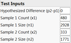
Check the box to paste in 2 columns of data (stacked or unstacked) and press Use Data or specify the sample sizes and either the sample counts or the sample proportions and press Calculate.
🔗

🔗
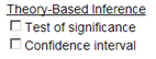
For the test, check the box for Test of Significance. Keep the hypothesized difference at zero and set the direction of the alternative, press Calculate.
🔗

🔗
For the confidence interval, check the Confidence Interval box, specify the confidence level and press Calculate CI
🔗

🔗

🔗

Hint 2. R Instructions

The iscamtwopropztest function takes the following inputs:

🔗

observed1 = either the number of successes or sample proportion for first group
🔗

🔗
n1 = sample size for first group
🔗

🔗
observed2 = count or proportion for second group
🔗

🔗
n2 = sample size for second group
🔗

🔗
hypothesized = hypothesized difference (default is 0)
🔗

🔗
alternative = "less", "greater", or "two.sided" for the direction of the alternative hypothesis
🔗

🔗
conf.level = the confidence level (e.g., 0.95 for 95%)
🔗

🔗

🔗

For the hearing loss study:

🔗

This finds the p-value for a one-sided alternative as well as a 95% confidence interval for \(\pi_1-\pi_2\text{.}\)

🔗

Hint 3. JMP Instructions

With raw data or after specifying the two-way table in column format, select Analyze > Fit Y by X and specify the categorical response variable (Y, Response) and the categorical explanatory variable (X, Factor)
🔗

🔗
Press OK.
🔗

🔗

🔗

The p-value in the Pearson row matches a two-sided z-test.

🔗
For a confidence interval, use the hot spot to select Two Sample Test for Proportions

🔗

Note: Here you can change which outcome is considered success. This also reports an "adjusted Wald" p-value

🔗

With summary data use the ISCAM Journal file: Hypothesis Test for Two Proportions
🔗

🔗
Specify the form of the alternative hypothesis
🔗

🔗
Enter the number of successes and the sample sizes
🔗

🔗

🔗

(This works for raw data too, but be careful how you specify the explanatory and response variables and use "pooled estimate of variance." This reports the z-score as well.)

🔗

Note: Data are "stacked" if each column represents a different variable (e.g., year surveyed and hearing condition) and they are "unstacked" if each column represents a different group (e.g., 1998 and 2002).

🔗

Subsection 13.1.2 Practice Problem 3.1A

In a follow-up study, Su & Chan (2017) examined hearing loss data for 1165 participants from the 2009-2010 National Health and Nutrition Examination Survey to see whether this trend has continued. They estimate the prevalence (after adjusting for a non-simple random sample and weighting the data to be representative of the population) of some hearing loss to be 0.152. If we treat this as a sample proportion, is this significantly different from the 2005-6 data?

🔗

Checkpoint 13.1.28.

Analyze whether the 2009-2010 data is significantly different from the 2005-6 data.

🔗

Subsection 13.1.3 Practice Problem 3.1B

In Practice Problem 1.1B, you considered data on the first 3 months of the Premier soccer league in 2019 (pre-Covid) and in 2020 (during Covid, when no fans were allowed). Consider these observations as random samples from independent processes. In 2019, the home team won 54 of the first 88 games and in 2020, the home team won 40 of 87 matches.

🔗

Checkpoint 13.1.29. Two-Way Table.

Create the two-way table for comparing these samples to each other. Calculate and interpret the difference in conditional proportions.

🔗

Checkpoint 13.1.30. Hypotheses.

Specify appropriate null and alternative hypothesis, being clear how these hypotheses change from Chapter 1. Are you using a one-sided or two-sided alternative?

🔗

Checkpoint 13.1.31. Simulation.

Use the Comparing Two Population Proportions applet to carry out a simulation. What are you using for the common probability of success? Which values do you count for the p-value? What do you conclude?

🔗

Checkpoint 13.1.32. Technical Conditions.

Are the technical conditions met to calculate the two-sample \(z\)-interval for these data? Explain.

🔗

Checkpoint 13.1.33. Confidence Interval.

Calculate and interpret a 95% confidence interval from these data.

🔗

Technology Detour – Simulating Proportions from Independent Random Samples.

🔗

Simulation Steps:

🔗

Generate a random sample of 2928 observations from a binomial process with \(\pi = .173\)
🔗

🔗
Generate a random sample of 1771 observations from a binomial process with \(\pi = .173\)
🔗

🔗
Convert the sample counts into sample proportions
🔗

🔗
Calculate the difference in the sample proportions
🔗

🔗
Repeat steps 1-4 a large number of times.
🔗

🔗

🔗

You should explore the individual \(\hat{p}\) distributions but most focus on the distribution of \(\hat{p}_1 - \hat{p}_2\text{,}\) including the mean, standard deviation, and whether the distribution behaves like a normal distribution.

🔗

Hint 1. R Instructions

Generate a random sample for 1994:

🔗

Generate 1000 random samples from each year, calculate the proportions, find the differences:

🔗

Display the generated distributions:

🔗

Compare to a normal distribution:

🔗

Hint 2. JMP Instructions

Generate a random sample for 1994:

🔗

In an empty Data window, select Cols > New Column. Name the column count1994, and specify 1 row. Create a formula and select Random > Random Binomial. Specify n = 2928 and p = 0.173. Press OK
🔗

🔗

🔗

Generate 1000 random samples from each year, calculate the proportions, find the differences:

🔗

Create a new column but specify 1000 as the number of rows and repeat the above commands. (After creating the first column, you can double click on a second column to activate it, and then right click to open the formula editor.)
🔗

🔗
Then create a new column/formula where you compute the difference in the proportions: count1994/2928 – count2006/1771. Call this column diff.
🔗

🔗

🔗

Display the generated distributions:

🔗

Choose Analyze > Distribution and specify the differences column.
🔗

🔗
Create a new column with a "conditional if" formula for diff \(\leq\) -0.024 ("true" or "false"). Then use Analyze > Distribution to tally this column.
🔗

🔗

🔗

Compare to a normal distribution:

🔗

Use the diff hot spot to select Continuous Distribution > Normal and to select Normal Quantile Plot.
🔗

🔗

🔗

You have attempted of activities on this page.

🔗

Prev Top Next