Investigation 1.3: Are You Clairvoyant?

Section 2.3 Investigation 1.3: Are You Clairvoyant?

A standard test for extra-sensory perception (ESP) asks subjects to identify which of five symbols (e.g., circle, plus, square, diamond, waves) is on the front of a card, viewed by the experimenter but not the subject. The experimenter concentrates on the symbol and a “hit” is when the subject correctly identifies the symbol being viewed by the experimenter. The subject is given several trials, with the viewed symbol randomly determined for each of the trials, with no discernible pattern.

🔗

ESP Test Symbols:

🔗

Online tests are available as well. Go to www.psychicscience.org/esp3.aspx to test your clairvoyance (predicting what’s about to happen rather than reading what someone else is thinking). Scroll down to Advanced ESP Test and review the 5 possible symbols, then press Start. Click on the card that you believe is about to be shown. Repeat for 10 rounds, keeping tracking of the number of hits in your first 10 attempts.

🔗

Checkpoint 2.3.1. Conduct the ESP Test.

How many hits did you get?

🔗

Checkpoint 2.3.2. Identify Sample and Variable.

Identify the sample and variable for this random process.

🔗

Hint.

What is the sample size? What was measured about each observation?

🔗

Solution.

The random process is the repeated attempts to identify the symbol correctly. The sample size is the 10 trials. Variable = correct/incorrect identification (categorical). The sample size is 10.

🔗

Checkpoint 2.3.3. Binomial Random Process.

Do you consider it reasonable to model your observations as coming from a binomial random process? Explain your reasoning.

🔗

Hint.

Consider the four conditions for a binomial process: two outcomes, independence, fixed number of trials, and constant probability.

🔗

Solution.

If the target symbols are randomly selected (equally likely), the student uses the same method each time, and the student is not more likely to correctly identify some symbols more than others (e.g., guessing each time) then a binomial process does seem reasonable.

🔗

Terminology Detour: Statistic vs. Parameter.

In analyzing data, it is important to differentiate between a statistic and the parameter. The observed statistic is a (known) numerical value that summarizes the observed results, whereas the parameter is the same numerical summary but applied to the underlying random process that generated the data. The value of the statistic is what we observe in the study, whereas the value of the parameter is rarely known.

🔗

In Investigation 1.1, the statistic could be either the number (14) or the proportion (0.875) of infants who chose the helper toy. The parameter would then be the long-run probability of an infant picking the helper toy. In the case of a binomial random variable, we will use the symbol \(\pi\) (lower case Greek letter for “p”) to represent this unknown process probability.

🔗

Checkpoint 2.3.4. Identify the Parameter.

Identify (in words) the parameter of interest for this study.

🔗

Hint.

A parameter describes a long-run probability or proportion for the entire process, not just your sample result.

🔗

Solution.

The parameter is your probability of correct identification (the long-run probability of correctly identifying the symbol).

🔗

Checkpoint 2.3.5. Parameter Symbol.

What symbol will we use to represent this parameter?

🔗

\(\hat{p}\)
This is the symbol for the sample proportion (statistic), not the population parameter.
\(\pi\)
Correct! We use \(\pi\) to represent the probability of success in a binomial process.
\(\mu\)
This is the symbol for a population mean, not a probability.
p
While p is sometimes used for probability, we use the Greek letter \(\pi\) for the process probability parameter.

Hint.

Look for the Greek letter used for a process probability in a binomial distribution.

🔗

Solution.

We use \(\pi\) to represent your probability of correct identification.

🔗

Checkpoint 2.3.6. State the Null Hypothesis.

The null hypothesis is that you aren’t clairvoyant and are guessing every time. State this as a null hypothesis using symbols and words.

🔗

Tip: Type "pi" for the Greek letter. Format as: H_0: pi = value

🔗

Hint.

If guessing randomly among 5 symbols, what is the probability of guessing correctly?

🔗

Solution.

\(H_0: \pi = 0.20\) (you have a 1 in 5 chance of guessing correctly)

🔗

Checkpoint 2.3.7. State the Alternative Hypothesis.

State the alternative hypothesis using symbols and words.

🔗

Tip: Type "pi" for the Greek letter. Use greater than, less than, or not equal to. Format as: H_a: pi > value

🔗

Aside

Hint.

If you are clairvoyant, would your probability of correct identification be higher or lower than random guessing?

🔗

Solution.

\(H_a: \pi > 0.20\) (you have a higher probability of predicting correctly)

🔗

Checkpoint 2.3.8. Simulation Method.

Assume the null hypothesis is true and let the random variable \(C\) denote the number of correct identifications (hits) in 10 attempts. If we were to simulate this random process, could we toss coins? If not, suggest another way we could generate simulated results assuming the null hypothesis to be true. (e.g., what would you want an applet to do?)

🔗

Hint.

Coin tosses give 50/50 probability. Does your null hypothesis assume 50% chance of success?

🔗

Solution.

We can model \(C\) with the binomial distribution:

🔗

Each trial has two outcomes: correct match or not
🔗

🔗
The trials are independent (the cards are shuffled in between attempts and the symbols are placed at random with no patterns from trial to trial)
🔗

🔗
There are a fixed number of attempts (\(n = 10\))
🔗

🔗
The probability of success (if someone is guessing) is the same for each trial (\(= 0.20\) if using 5 cards each trial). We aren’t changing the number of cards or anything else from trial-to-trial.
🔗

🔗

🔗

We can’t toss a coin because we are not assuming 50/50 for success/failure. To model 0.20 we could use spinners.

🔗

Checkpoint 2.3.9. Null Distribution Predictions.

Where do you think your null distribution will be centered? What are the largest and smallest possible values for the number of correct identifications in 10 attempts? What are the largest and smallest values you think you will see in the simulation?

🔗

Hint.

Use the probability from the null hypothesis times the number of attempts to find the expected value.

🔗

Solution.

On average, if someone is guessing, we would “expect” to see \(\frac{1}{5}(10) = 2\) correct answers (in the long run). \(E(C) = 10(0.20) = 2\) if assuming 5 cards.

🔗

Checkpoint 2.3.10. Carry Out the Simulation.

In the One Proportion Inference applet, specify the values for \(\pi\) and \(n\text{.}\) Carry out one repetition of the simulation. Explain the simulation process in your own words.

🔗

Hint.

Set pi to your null hypothesis value and n to the number of attempts you made.

🔗

Solution.

Results will vary. The applet should generate 10 spinners (each a 0.20 probability of success = landing in the blue region) and then record the number of successes in those 10 spins.

🔗

Checkpoint 2.3.11. Theoretical Mean and Standard Deviation.

Then check the Exact Binomial box to see the null distribution after infinitely many repetitions. Press the Reset button to remove the one simulated result and check the Summary Statistics box. What are the theoretical values for the mean and standard deviation of the null distribution?

🔗

Mean =

🔗

Std Dev =

🔗

Hint.

Look for the values displayed in the Summary Statistics section of the applet after pressing Reset.

🔗

Solution.

After pressing Reset to remove the one simulated trial, you should find Mean = 2.000, SD = 1.265.

🔗

Binomial Distribution Formulas.

It can be shown that when \(X\) is Binomial(\(n\text{,}\) \(\pi\)), the expected value is \(E(X) = n \times \pi\) and the variance is \(V(X) = n\pi(1 - \pi)\text{.}\) (See Exploration B for more discussion of expected value and variance of a random variable.)

🔗

Checkpoint 2.3.12. Verify the Calculations.

Verify these calculations match the applet output and remember that the standard deviation is the square root of the variance.

🔗

Hint.

Use the formulas provided in the previous question with n=10 and pi=0.20.

🔗

Solution.

\(E(C) = 10(0.2) = 2.00\) and \(SD(C) = \sqrt{10 \times 0.2 \times 0.8} = 1.265\text{.}\)

🔗

Checkpoint 2.3.13. Result in the Tail?

Was your statistic from Checkpoint 3.77 (your number of hits) in the direction specified by the alternative hypothesis? If it was, is it in one of the tails (outer edges) of the null distribution from Checkpoint 3.86?

🔗

Hint.

Compare your number of hits to the mean of the distribution. Is it larger (right tail) or smaller (left tail)?

🔗

Solution.

Results will vary, but quite possible your results were below the expected value.

🔗

If your observed number of successes was below the mean, then you can conclude that your data do not provide evidence in favor of the alternative hypothesis and you should not start your own psychic hotline! But if your result was above the mean, then we would like to measure the strength of evidence against the null hypothesis. You have already seen how to do that using a p-value.

🔗

Checkpoint 2.3.14. Explore p-value Threshold.

Use the applet to explore how many hits a subject would need in 10 attempts for the p-value to be below 0.05.

🔗

Hint.

Use your mouse to drag the red line.

🔗

Solution.

A subject would need at least 5 hits in 10 attempts for the p-value to be below 0.05 (specifically, P(X ≥ 5) = 0.0328).

🔗

An Alternative Measure of Rareness.

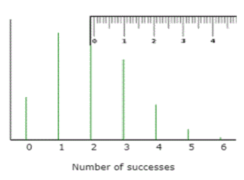
As an alternative to the p-value, another measure of where an observation falls in a distribution is “how many standard deviations” it is from the mean of the distribution.

🔗

A number line showing distances from the null hypothesis mean:

🔗

A ruler or number line showing the distance scale for evaluating deviations from the hypothesized mean.

\begin{equation*} \frac{\text{observed number of hits} - \text{expected value}}{\text{standard deviation}} \end{equation*}

🔗

Checkpoint 2.3.15. Standardize Your Result.

How many standard deviations was your observed result from the expected value for the binomial distribution?

🔗

Hint.

Use the formula: (observed - expected) / standard deviation. Substitute your number of hits for observed, and use the mean and SD from Checkpoint 3.86.

🔗

Solution.

The standardized statistic expresses the distance in “standard deviations away” from the hypothesized value of \(\pi\text{.}\) A negative value means the distance is below the mean; a positive value means the distance is above the mean.

🔗

This calculation is often referred to as standardizing the statistic.

🔗

Again, there are no hard and fast rules for what constitutes a large value here, but generally, when we have a fairly symmetric distribution, values more than 2 standard deviations above or below the expected value (mean) are considered extreme.

🔗

Checkpoint 2.3.16. Standardizing 5 Hits.

How many standard deviations from the mean (expected value) would 5 hits be?

🔗

Hint.

Use the same formula as the previous question: (5 - 2) / 1.265. What does this value tell you?

🔗

Solution.

A standardized statistic of 1 means that the sample result is one standard deviation above the mean of 2. Because the SD is 1.265, 1 SD above the mean is at \(2 + 1.265 = 3.265\text{.}\) Rounding to the nearest whole number, that would correspond to 3 correct identifications. (Or you could solve: \((x - 2)/1.265 = 1\) to find \(x = 3.265\text{.}\))

🔗

Checkpoint 2.3.17. Distribution for 25 Attempts.

Suppose you don’t know whether or not someone is clairvoyant and you plan to give the person 25 attempts. What are the theoretical expected number and standard deviation for the random variable \(C\text{,}\) the number of hits when \(n = 25\) assuming they are just guessing each time? How do they compare to the values you found in (j)?

🔗

Hint.

Use the binomial formulas with n = 25 and pi = 0.20. Expected value = n × pi, and SD = square root of n × pi × (1 - pi).

🔗

Solution.

Expected value = \(5\text{,}\) SD = \(2\)

🔗

Note: You can check these in the applet. Because the value of \(n\) has changed, both have increased. The larger the sample size, the more variability in the distribution.

🔗

How many hits would someone need to get correct in 25 attempts to convince you they aren’t simply guessing? Let’s consider two ways to decide.

🔗

Checkpoint 2.3.18. Approach 1: P-value Threshold.

Approach 1: What value for \(c\) would give you a probability below 0.05 of obtaining that many or more hits? In other words, what is the smallest value of \(c\) so \(P(C \geq c) < 0.05\text{?}\)

🔗

Hint.

Use the applet to find probabilities for different values of c.

🔗

Solution.

We need to find \(c\) such that \(P(C \geq c) < 0.05\text{.}\) Using the applet:

\(P(C \geq 8) = 0.109\) (too large)
🔗

🔗
\(P(C \geq 9) = 0.048\) (this will work!)
🔗

🔗

So if someone had 9 or more correct, we might choose to consider that statistically significant.

🔗

Checkpoint 2.3.19. Approach 2: Standard Deviations.

Approach 2: What is the smallest value of \(c\) that is at least 2 standard deviations from the expected value?

🔗

Hint.

Use the expected value and standard deviation from Checkpoint 3.93.

🔗

Solution.

The observed value would need to be more than \(5 + 2(2) = 9\text{.}\)

🔗

Checkpoint 2.3.20. Compare the Two Approaches.

How do your answers for these two approaches compare?

🔗

Hint.

Look at the values of c you found in both approaches. Are they the same or very close? What does this suggest about the relationship between p-values and standard deviations?

🔗

Solution.

It is not a coincidence that the value of 9 appears in both and is close to the expected value + 2 SD. It turns out that with a “large enough” sample size, if a standardized statistic is about 2 SD from the mean, the p-value will be close to 0.05. We will develop this idea much more carefully when we turn to the normal approximation to the binomial.

🔗

Checkpoint 2.3.21. Test with Four Symbols.

Suppose you changed the test to use only 4 symbols. Does this change the expected number or standard deviation for the number of hits when a subject is guessing? How many would someone need to identify correctly to convince you they could perform better than guessing in the long-run?

🔗

Hint.

With 4 symbols, the probability of guessing correctly changes to 1/4 = 0.25. Recalculate the expected value and SD using this new probability, then find how many hits would be 2 SD above the mean.

🔗

Solution.

This would increase the probability of a correct guess to 0.25, and so the probability model would need to change as well. If there are only 4 cards, the probability of a correct guess increases to 0.25. So, with 25 attempts, the expected value would be \(25(0.25) = 6.25\) with an SD of \(\sqrt{25(0.25)(0.75)} = 2.17\text{.}\) So \(6.25 + 2(2.17) = 10.59 \approx 11\text{.}\) Notice that this “cutoff” value went up (10 or 11 vs. 9). This is because guessing is more likely to do well so we need more evidence that someone is not guessing. Also, using the applet, \(P(C \geq 10) = 0.097\) and \(P(C \geq 11) = 0.044\text{.}\)

🔗

Summary.

The number of correct answers in 25 attempts, for someone who is guessing, can be modeled with a binomial distribution (assuming the probability of a correct answer is 0.20 each time and there is no pattern from attempt to attempt). In this case, the hypothesized value for the probability of “success” will be 0.20 rather than 0.5 due to the five cards to choose from, which we could model with spinners rather than coin tosses. If someone is simply guessing, in the long run they will guess correctly by chance alone 20% of the time. This means that if we give someone 25 attempts, we expect them to answer correctly \(0.20 \times 25 = 5\) times (on average, in the long run), with a standard deviation of \(\sqrt{25(0.20)(0.80)} = 2\) hits in 25 attempts. Keep in mind that the “statistical significance” of an outcome will depend on both the mean and the standard deviation of the null distribution. In this case, someone would need 9 or more hits to be more than 2 standard deviations above the mean, which corresponds to a p-value of 0.048. (It is not a coincidence that the 0.05 cut-off gives very similar results to the 2SD cut-off.)

🔗

Subsection 2.3.1 Practice Problem 1.3A

Checkpoint 2.3.22. Six Symbols: Distribution Changes.

Suppose the test had consisted of 6 symbols instead of 5 (with \(n = 25\) still). How will that change the binomial distribution? [You should comment on both the mean and the standard deviation.]

🔗

Checkpoint 2.3.23. Six Symbols: Surprising Outcome.

Would an outcome of 9 correct guesses be more or less surprising in this case (vs. 5 symbols)?

🔗

Will the probability of 9 or more correct identifications be larger or smaller than with 5 symbols?
🔗

🔗
Will the outcome of 9 be more or fewer standard deviations from the mean than with 5 symbols?
🔗

🔗

🔗

Checkpoint 2.3.24. Ten Symbols.

What about 10 symbols? What are the mean and standard deviation of the binomial distribution? Would an outcome of 9 or more correct identifications be more or less surprising than with 5 symbols?

🔗

Checkpoint 2.3.25. Shape of Distribution.

How does the shape of the binomial distribution change as you lower \(\pi\text{?}\) Explain why.

🔗

Subsection 2.3.2 Practice Problem 1.3B

Return to the wolf (Yukon). In another study, Yukon correctly understood a communicative cue in 7 of 8 attempts.

🔗

Checkpoint 2.3.26. Parameter and Statistic.

Identify (in words) the parameter and statistic in that study.

🔗

Checkpoint 2.3.27. Standardized Result.

How many standard deviations did the observed statistic fall above the expected value assuming Yukon picks equally between the two containers regardless of the cue in the long run?

🔗

Checkpoint 2.3.28. Surprising Outcome?

Would her performance be considered a surprising outcome when the null hypothesis is true? Explain.

🔗

Return to the infants choosing a helper toy over a hinderer toy 14 times out of 16 choices.

🔗

Checkpoint 2.3.29. Infant Study: Parameter and Statistic.

Identify (in words) the parameter and statistic in that study.

🔗

Checkpoint 2.3.30. Infant Study: Standardized Result.

How many standard deviations did the observed statistic fall above the expected value assuming infants choose equally between the two types of toys?

🔗

Checkpoint 2.3.31. Infant Study: Time Variable.

In the infant study, researchers also looked at the amount of time the infants spent watching the two videos (to see whether one captured their attention more than the other). Identify a possible parameter of interest for this new variable.

🔗