Investigation 1.7: Reese’s Pieces (Optional)

Section 3.1 Investigation 1.7: Reese’s Pieces (Optional)

Manufacturers often perform "quality checks" to ensure that their manufacturing process is operating under certain specifications. Suppose a manager at Hershey’s is concerned that his manufacturing process is no longer producing the correct color proportions (orange, yellow, brown) in Reese’s candies.

🔗

Checkpoint 3.1.1. (a) Initial Prediction.

Prediction: A friend finds 10 orange candies in her bag. Does this convince you that the three colors are not equally likely? What other information would you want to know? What if she tells you these orange pieces were 50% of the candies in her bag?

🔗

Hint.

Consider: Knowing the total number of candies in the bag is crucial. What’s the difference between 10 out of 20 versus 10 out of 100?

🔗

Solution.

Conjectures will vary. Knowing the total number of candies (sample size) is crucial. 10 out of 20 (50%) is much different from 10 out of 100 (10%). With 50% orange, this provides some evidence against equal proportions, but we would want more information about sampling variability.

🔗

Checkpoint 3.1.2. (b) Record Your Sample.

Take a (presumably representative) sample of n = 25 Reese’s Pieces candies and record the number of orange, yellow, and brown candies in your sample.

🔗

Orange: Yellow: Brown:

🔗

Solution.

Results will vary. Students should record their data and be prepared to share it with the class.

🔗

Checkpoint 3.1.3. (c) Identify Sample and Variable.

Identify the sample/random process and variable for your sample.

🔗

Sample/Random process:

🔗

Variable:

🔗

Type:

🔗

Hint.

The random process is selecting candies. The variable is the color of each candy. Is this categorical or quantitative?

🔗

Solution.

Sample/Random process: The random process is selecting Reese’s Pieces candies.

🔗

Variable: The color of each candy

🔗

Type: Categorical (with three possible values: orange, yellow, brown)

🔗

Checkpoint 3.1.4. (d) Assess Binomial Process.

Define "success" to be an orange candy and "failure" to be a non-orange candy. Is it reasonable to treat these data as observations from a binomial process? Explain.

🔗

Hint.

Consider: Are there two possible outcomes? Fixed number of trials? Independent trials? Constant probability of success?

🔗

Solution.

Yes, this is reasonably a binomial process: There are two possible outcomes (orange/not orange), a fixed number of trials (n = 25), the trials are independent (assuming sampling with replacement or from a very large population), and the probability of success (getting an orange candy) is constant for each trial. The main assumption to consider is whether the candies are well-mixed and randomly selected.

🔗

Checkpoint 3.1.5. (e) Initial Assessment.

Prediction: Based on your data, do you think one-third is a plausible value for the probability Hershey’s process produces an orange candy? How are you deciding? What more information do you need?

🔗

Solution.

Conjectures will vary. Students need more information about how much variability to expect in sample proportions when the true probability is one-third. A simulation will help determine whether the observed sample proportion is reasonably close to 1/3 or surprisingly far away.

🔗

Reporting the sample proportion as the statistic is often more informative than the sample count, but that means we need to know about the null distribution of sample proportions.

🔗

Checkpoint 3.1.6. (f) Initial Simulation.

Open the Reese’s Pieces applet.

🔗

Set the applet to assume a 0.333 process probability of a Reese’s Pieces candy being orange. The applet is set to take a sample of n = 25 candies.

🔗
Click the Draw Samples button.

🔗
The applet will randomly select a sample of 25 candies, sort them, and report the sample number of orange candies.

🔗
Click the Draw Samples button again.

🔗

🔗

Did you get the same number of orange candies both times?

🔗

Solution.

No, you typically get different numbers of orange candies. This demonstrates sampling variability—even when the true probability is 0.333, individual samples produce different results due to random chance.

🔗

Checkpoint 3.1.7. (g) Interpret Dotplot.

Change the Number of samples from 1 to 1998.

🔗
Uncheck the Show animation box.

🔗
Click the Draw Samples button again.

🔗
Select the Proportion of orange radio button.

🔗
What does each dot in this dotplot represent?

🔗

🔗

Hint.

Each dot represents the sample proportion of orange candies in one sample of 25 candies.

🔗

Solution.

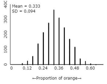
Each dot represents the sample proportion of orange candies in one sample of 25 candies. The entire dotplot shows the distribution of sample proportions across many samples when the true probability is 0.333, illustrating the sampling distribution of the sample proportion.

🔗

Dotplot showing the distribution of sample proportions for n=25 candies with probability 0.333

🔗

Binomial Random Variable Properties.

Recall that for a binomial random variable, \(X\text{,}\) the expected value \(E(X) = n \times \pi\) and the standard deviation \(SD(X) = \sqrt{n \times \pi \times (1-\pi)}\text{.}\) It can also be shown that random variables follow these rules:

🔗

For any constant \(c\text{,}\) \(E(cX) = c \times E(X)\)

🔗
For any constant \(c\text{,}\) \(SD(cX) = |c| \times SD(X)\)

🔗

🔗

Checkpoint 3.1.8. (h) Derive Formulas.

Use the above information, and the fact that \(\hat{p} = X/n\text{,}\) to derive formulas for \(E(\hat{p})\) and \(SD(\hat{p})\text{.}\)

🔗

Hint.

Start with \(E(\hat{p}) = E(X/n) = E((1/n) \times X)\) and apply the rule for constants.

🔗

Solution.

\(E(\hat{p}) = E(X/n) = (1/n) \times E(X) = (1/n) \times n\pi = \pi\)

🔗

\(SD(\hat{p}) = SD(X/n) = (1/n) \times SD(X) = (1/n) \times \sqrt{n\pi(1-\pi)} = \sqrt{\frac{\pi(1-\pi)}{n}}\)

🔗

Mathematical formulas for expected value and standard deviation of sample proportion

🔗

Checkpoint 3.1.9. (i) Verify Formulas.

Using \(\pi = 0.333\) and \(n = 25\text{,}\) verify that your formulas match the results from checking the Summary Statistics box in the applet.

🔗

Hint.

Calculate \(E(\hat{p}) = 0.333\) and \(SD(\hat{p}) = \sqrt{\frac{0.333(0.667)}{25}}\)

🔗

Solution.

\(E(\hat{p}) = \pi = 0.333\)

🔗

\(SD(\hat{p}) = \sqrt{\frac{\pi(1-\pi)}{n}} = \sqrt{\frac{0.333(0.667)}{25}} = \sqrt{\frac{0.222}{25}} = \sqrt{0.00888} \approx 0.094\)

🔗

These values should match the mean and standard deviation shown in the applet’s summary statistics.

🔗

Checkpoint 3.1.10. (j) Predict Larger Sample.

Prediction: If we had instead taken 2,000 samples of size n = 100 candies, how do you think the distribution of the sample proportions would compare to the distribution where n = 25? Explain.

🔗

Hint.

Think about how sample size affects variability in sample proportions.

🔗

Solution.

With n = 100, we would expect less variability in the sample proportions compared to n = 25. The distribution should still be centered at 0.333 and roughly symmetric, but with much less spread. Larger sample sizes lead to more precise estimates of the population parameter.

🔗

Checkpoint 3.1.11. (k) Compare Distributions.

In the applet:

Without pressing Reset, change the Number of candies in the applet to 100.

🔗
Change the Number of samples to 2,000.

🔗
Press Draw Samples to generate a new distribution.

🔗
Check the Show previous results box to display the previous distribution in the background in light grey.

🔗
Describe the behavior (shape, center, variability) of this (new) distribution and how it has changed from the previous.

🔗

🔗

Focus on the most substantial change in the distribution. Is this what you expected?

🔗

Hint.

Pay special attention to the spread of the distribution - how has it changed?

🔗

Solution.

The center remains at approximately 0.333. The shape remains roughly symmetric and mound-shaped. The most substantial change is in variability: the distribution with n = 100 has much less spread than the distribution with n = 25. This makes sense because larger sample sizes lead to less sampling variability.

🔗

Comparison of sampling distributions for n=25 and n=100 showing reduced variability with larger sample size

🔗

Checkpoint 3.1.12. (l) Smaller Sample Size.

Repeat the previous questions (using the formulas, checking against the applet) for a sample size of n = 5 candies.

🔗

Hint.

Calculate the expected value and standard deviation for n = 5, then compare the distribution to n = 25.

🔗

Solution.

For n = 5:

🔗

\(E(\hat{p}) = \pi = 0.333\)

🔗

\(SD(\hat{p}) = \sqrt{\frac{0.333(0.667)}{5}} = \sqrt{0.0444} \approx 0.211\)

🔗

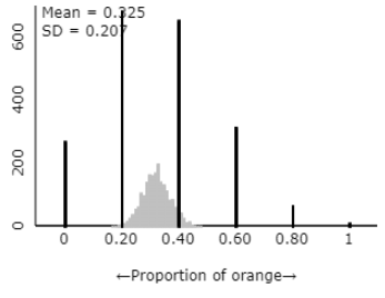
The distribution with n = 5 has much more variability (SD ≈ 0.211) compared to n = 25 (SD ≈ 0.094). The center remains at 0.333, but smaller sample sizes produce much more spread in the sample proportions.

🔗

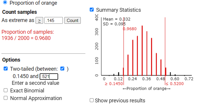
Checkpoint 3.1.13. (m) Calculate Cut-offs.

Return to the scenario where n = 25 and \(\pi = 0.333\text{.}\) Earlier, you predict that in this scenario \(E(\hat{p}) = 0.333\) and \(SD(\hat{p}) = 0.094\text{.}\) Calculate the following "cut-offs":

🔗

\(\pi - 2 \times SD(\hat{p})\) = and \(\pi + 2 \times SD(\hat{p})\) =

🔗

Solution.

\(\pi - 2 \times SD(\hat{p}) = 0.333 - 2(0.094) = 0.333 - 0.188 = 0.145\)

🔗

\(\pi + 2 \times SD(\hat{p}) = 0.333 + 2(0.094) = 0.333 + 0.188 = 0.521\)

🔗

These values represent the boundaries within which approximately 95% of sample proportions should fall when \(\pi = 0.333\) and \(n = 25\text{.}\)

🔗

Checkpoint 3.1.14. (n) Percentage Within Two Standard Deviations.

Use the applet to determine the percentage of samples with a sample proportion within 2 standard deviations of the expected value.

🔗

Set the probability of orange to 0.333 and the number of candies to 25.

🔗
Generate 2,000 samples.

🔗
Enter the first value from (m) in the As extreme as box.

🔗
Check the Two-tailed box and then the between box.

🔗
Enter the second value in the box that appears.

🔗

🔗

Write a sentence reporting the percentage of samples with a proportion of orange candies between these two values.

🔗

Hint.

The percentage should be close to 95%.

🔗

Solution.

Approximately 95-96% of the samples have a sample proportion between 0.145 and 0.521 (within two standard deviations of 0.333). This percentage may vary slightly in different simulations due to random chance, but should consistently be close to 95%.

🔗

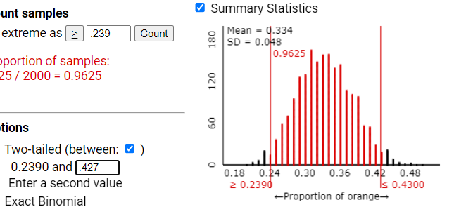
Distribution showing approximately 95% of sample proportions falling within two standard deviations of the mean

🔗

Checkpoint 3.1.15. (o) Compare for n = 100.

Repeat the previous two questions (calculating cut-offs and using the applet to find the percentage) for n = 100 (including using the new SD and new cut-offs). How does the percentage of samples within two standard deviations of 0.333 compare?

🔗

Hint.

The percentage should still be close to 95%, regardless of sample size.

🔗

Solution.

For n = 100: \(SD(\hat{p}) = \sqrt{\frac{0.333(0.667)}{100}} \approx 0.047\)

🔗

Cut-offs: \(0.333 \pm 2(0.047)\) gives (0.239, 0.427)

🔗

The percentage of samples within these cut-offs is still approximately 95%. While the standard deviation is smaller (less variability), the percentage within two standard deviations remains consistent regardless of sample size. This demonstrates that the empirical rule applies to the sampling distribution regardless of sample size.

🔗

Definition: The Empirical Rule.

The Empirical Rule or the 68-95-99.7 rule states that for a mound-shaped, symmetric distribution:

🔗

the interval (mean – SD, mean + SD) should capture approximately 68% of the distribution.

🔗
the interval (mean – 2 SD, mean + 2 SD) should capture approximately 95% of the distribution.

🔗
the interval (mean – 3 SD, mean + 3 SD) should capture approximately 99.7% of the distribution.

🔗

🔗

Checkpoint 3.1.16. (p) Verify Empirical Rule.

Do your simulation results agree with the empirical rule?

🔗

Solution.

Yes, the simulation results agree well with the empirical rule. Approximately 95% of the sample proportions fall within two standard deviations of the mean (0.333), which is consistent with the empirical rule’s prediction for mound-shaped, symmetric distributions.

🔗

Checkpoint 3.1.17. Complete Statements.

Complete the following statements:

🔗

Roughly % of sample proportions fall within of the value of \(\pi\text{.}\)

🔗

For roughly % of samples, \(\pi\) falls within of any sample proportion.

🔗

Hint.

Think about the empirical rule and standard deviations.

🔗

Solution.

Roughly 95% of sample proportions fall within 2 SD of the value of \(\pi\text{.}\)

🔗

For roughly 95% of samples, \(\pi\) falls within 2 SD of any sample proportion.

🔗

Discussion.

Notice that if we know the value of \(\pi\) and we know the sample size n, we can predict the value of the sample proportion fairly precisely. This will be very helpful to us in deciding whether an observed sample proportion is "far away" from a hypothesized value for \(\pi\text{.}\)

🔗

Subsection 3.1.1 Practice Problem 1.7A

Checkpoint 3.1.18. Sample Proportions Range.

In this investigation, you took samples of 25 candies. 95% of the sample proportions should fall between and when \(\pi = 0.50\text{.}\)

🔗

Hint.

Use the empirical rule: approximately 95% of values fall within 2 standard deviations of the mean.

🔗

Solution.

With n = 25 and π = 0.50, the standard deviation is sqrt(0.50 × 0.50 / 25) = 0.10. Using the empirical rule, 95% of sample proportions should fall between 0.50 - 2(0.10) = 0.30 and 0.50 + 2(0.10) = 0.70.

🔗

Subsection 3.1.2 Practice Problem 1.7B

An expert witness in a paternity suit testifies that the length (in days) of pregnancy (the time from conception to delivery of the child) is approximately normally distributed with mean \(\mu = 270\) days and standard deviation \(\sigma = 10\) days. The defendant in the suit is able to prove that he was out of the country during a period that began 280 days before the birth of the child and ended 230 days before the birth of the child.

🔗

Checkpoint 3.1.19. Normal Model Assumption.

Does a normal model seem to be a reasonable assumption here? Explain why or why not or how you might decide.

🔗

Checkpoint 3.1.20. Probability Calculation.

If the defendant was the father of the child, what is the probability that the mother could have had the very long (more than 280 days) or the very short (less than 230 days) pregnancy indicated by the testimony?

🔗

You have attempted of activities on this page.

🔗

Prev Top Next