Strayer and Johnston (2001) asked student volunteers to use a machine that simulated driving situations. At irregular intervals, a target would flash red or green. Participants were instructed to press a "brake button" as soon as possible when they detected a red light. The machine would calculate the reaction time to the red flashing targets for each student in milliseconds.
The students were given a warm-up period to familiarize themselves with the driving simulator. Then the researchers had each student use the driving simulation machine while talking on a cell phone about politics to someone in another room and then again with music or a book-on-tape playing in the background (control). The students were randomly assigned as to use the cell phone or the control setting for the first trial. The reaction times (in milliseconds) for 16 students appear below and in the file driving.txt.
Checkpoint11.2.1.Identify probability distribution and assumptions.
Suppose we let \(X\) represent the number of subjects whose cell phone reaction time was longer. What probability distribution can we use to model \(X\text{?}\) What assumptions are behind this probability model?
We can use the binomial distribution to model \(X\text{,}\) where \(n = 16\) (the number of drivers in the study) and \(\pi\) represents the probability that the cell phone reaction time is longer. This is a valid model as long as the reaction times between subjects are independent and the probability of the cell phone reaction time being longer is the same across the subjects.
Checkpoint11.2.3.Calculate observed value and describe evidence assessment.
What is the observed value of \(X\) in this study? How would you determine whether this statistic provides convincing evidence against the null hypothesis?
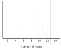
The observed value of \(X\) is 13 in this study. So we need to assess how unusual it is for 13 or more drivers out of 16 to have a longer cell phone reaction time under the null hypothesis that there is no long-run tendency for either reaction time to be longer.
Checkpoint11.2.4.Determine p-value and interpret results.
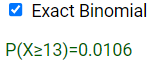
Use the binomial distribution to determine a p-value for a sign test applied to this study. Interpret this p-value in the context of this study and state the conclusions you would draw from this p-value.
With an exact Binomial p-value of 0.0106, we would reject the null hypothesis at the 5% level of significance. Only 1.1% of random assignments (of which reaction time goes to which condition for each person) would have at least 13 of the differences being positive if the null hypothesis were true. We have strong evidence that such a majority did not happen by chance alone, but reflects a genuine tendency for cell phone reaction times to be longer.