
Advanced High School Statistics: Third Edition

Section B.2 Normal Probability Table

A normal probability table may be used to find percentiles of a normal distribution using a Z-score, or vice-versa. Such a table lists Z-scores and the corresponding percentiles. An abbreviated probability table is provided in Table B.2.1 that we’ll use for the examples in this appendix. A full table may be found further below.
Table B.2.1. A section of the normal probability table. The percentile for a normal random variable with \(Z = 1.00\) has been emphasized, and the percentile closest to 0.8000 has also been bolded
Second decimal place of \(Z\)
\(Z\) 0.00 0.01 0.02 0.03 0.04 0.05 0.06 0.07 0.08 0.09
0.0 0.5000 0.5040 0.5080 0.5120 0.5160 0.5199 0.5239 0.5279 0.5319 0.5359
0.1 0.5398 0.5438 0.5478 0.5517 0.5557 0.5596 0.5636 0.5675 0.5714 0.5753
0.2 0.5793 0.5832 0.5871 0.5910 0.5948 0.5987 0.6026 0.6064 0.6103 0.6141
0.3 0.6179 0.6217 0.6255 0.6293 0.6331 0.6368 0.6406 0.6443 0.6480 0.6517
0.4 0.6554 0.6591 0.6628 0.6664 0.6700 0.6736 0.6772 0.6808 0.6844 0.6879
0.5 0.6915 0.6950 0.6985 0.7019 0.7054 0.7088 0.7123 0.7157 0.7190 0.7224
0.6 0.7257 0.7291 0.7324 0.7357 0.7389 0.7422 0.7454 0.7486 0.7517 0.7549
0.7 0.7580 0.7611 0.7642 0.7673 0.7704 0.7734 0.7764 0.7794 0.7823 0.7852
0.8 0.7881 0.7910 0.7939 0.7967 0.7995 0.8023 0.8051 0.8078 0.8106 0.8133
0.9 0.8159 0.8186 0.8212 0.8238 0.8264 0.8289 0.8315 0.8340 0.8365 0.8389
1.0 0.8413 0.8438 0.8461 0.8485 0.8508 0.8531 0.8554 0.8577 0.8599 0.8621
1.1 0.8643 0.8665 0.8686 0.8708 0.8729 0.8749 0.8770 0.8790 0.8810 0.8830
\(\vdots\) \(\vdots\) \(\vdots\) \(\vdots\) \(\vdots\) \(\vdots\) \(\vdots\) \(\vdots\) \(\vdots\) \(\vdots\) \(\vdots\)
When using a normal probability table to find a percentile for \(Z\) (rounded to two decimals), identify the proper row in the normal probability table up through the first decimal, and then determine the column representing the second decimal value. The intersection of this row and column is the percentile of the observation. For instance, the percentile of \(Z = 0.45\) is shown in row 0.4 and column 0.05 in Table B.2.1: 0.6736, or the 67.36th percentile.
Figure B.2.2. The area to the left of \(Z\) represents the percentile of the observation

Example B.2.3.

SAT scores follow a normal distribution, \(N(1100, 200)\text{.}\) Ann earned a score of 1300 on her SAT with a corresponding Z-score of \(Z = 1\text{.}\) She would like to know what percentile she falls in among all SAT test-takers.
Solution.
Ann’s percentile is the percentage of people who earned a lower SAT score than her. We shade the area representing those individuals in the following graph:
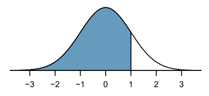
The total area under the normal curve is always equal to 1, and the proportion of people who scored below Ann on the SAT is equal to the area shaded in the graph. We find this area by looking in row 1.0 and column 0.00 in the normal probability table: 0.8413. In other words, Ann is in the 84th percentile of SAT takers.

Example B.2.4.

How do we find an upper tail area?
Solution.
The normal probability table always gives the area to the left. This means that if we want the area to the right, we first find the lower tail and then subtract it from 1. For instance, 84.13% of SAT takers scored below Ann, which means 15.87% of test takers scored higher than Ann.
We can also find the Z-score associated with a percentile. For example, to identify \(Z\) for the 80th percentile, we look for the value closest to 0.8000 in the middle portion of the table: 0.7995. We determine the Z-score for the 80th percentile by combining the row and column Z values: 0.84.

Example B.2.5.

Find the SAT score for the 80th percentile.
Solution.
We look for the are to the value in the table closest to 0.8000. The closest value is 0.7995, which corresponds to \(Z = 0.84\text{,}\) where 0.8 comes from the row value and 0.04 comes from the column value. Next, we set up the equation for the Z-score and the unknown value \(x\) as follows, and then we solve for \(x\text{:}\)
\begin{gather*} Z= 0.84 = \frac{x-1100}{200} \rightarrow x = 1268 \end{gather*}
The College Board scales scores to increments of 10, so the 80th percentile is 1270. (Reporting 1268 would have been perfectly okay for our purposes.)
For additional details about working with the normal distribution and the normal probability table, see Section 2.3.
Table B.2.6.
Second decimal place of \(Z\)
0.09 0.08 0.07 0.06 0.05 0.04 0.03 0.02 0.01 0.00 \(Z\)
0.0002 0.0003 0.0003 0.0003 0.0003 0.0003 0.0003 0.0003 0.0003 0.0003 \(-3.4\)
0.0003 0.0004 0.0004 0.0004 0.0004 0.0004 0.0004 0.0005 0.0005 0.0005 \(-3.3\)
0.0005 0.0005 0.0005 0.0006 0.0006 0.0006 0.0006 0.0006 0.0007 0.0007 \(-3.2\)
0.0007 0.0007 0.0008 0.0008 0.0008 0.0008 0.0009 0.0009 0.0009 0.0010 \(-3.1\)
0.0010 0.0010 0.0011 0.0011 0.0011 0.0012 0.0012 0.0013 0.0013 0.0013 \(-3.0\)
0.0014 0.0014 0.0015 0.0015 0.0016 0.0016 0.0017 0.0018 0.0018 0.0019 \(-2.9\)
0.0019 0.0020 0.0021 0.0021 0.0022 0.0023 0.0023 0.0024 0.0025 0.0026 \(-2.8\)
0.0026 0.0027 0.0028 0.0029 0.0030 0.0031 0.0032 0.0033 0.0034 0.0035 \(-2.7\)
0.0036 0.0037 0.0038 0.0039 0.0040 0.0041 0.0043 0.0044 0.0045 0.0047 \(-2.6\)
0.0048 0.0049 0.0051 0.0052 0.0054 0.0055 0.0057 0.0059 0.0060 0.0062 \(-2.5\)
0.0064 0.0066 0.0068 0.0069 0.0071 0.0073 0.0075 0.0078 0.0080 0.0082 \(-2.4\)
0.0084 0.0087 0.0089 0.0091 0.0094 0.0096 0.0099 0.0102 0.0104 0.0107 \(-2.3\)
0.0110 0.0113 0.0116 0.0119 0.0122 0.0125 0.0129 0.0132 0.0136 0.0139 \(-2.2\)
0.0143 0.0146 0.0150 0.0154 0.0158 0.0162 0.0166 0.0170 0.0174 0.0179 \(-2.1\)
0.0183 0.0188 0.0192 0.0197 0.0202 0.0207 0.0212 0.0217 0.0222 0.0228 \(-2.0\)
0.0233 0.0239 0.0244 0.0250 0.0256 0.0262 0.0268 0.0274 0.0281 0.0287 \(-1.9\)
0.0294 0.0301 0.0307 0.0314 0.0322 0.0329 0.0336 0.0344 0.0351 0.0359 \(-1.8\)
0.0367 0.0375 0.0384 0.0392 0.0401 0.0409 0.0418 0.0427 0.0436 0.0446 \(-1.7\)
0.0455 0.0465 0.0475 0.0485 0.0495 0.0505 0.0516 0.0526 0.0537 0.0548 \(-1.6\)
0.0559 0.0571 0.0582 0.0594 0.0606 0.0618 0.0630 0.0643 0.0655 0.0668 \(-1.5\)
0.0681 0.0694 0.0708 0.0721 0.0735 0.0749 0.0764 0.0778 0.0793 0.0808 \(-1.4\)
0.0823 0.0838 0.0853 0.0869 0.0885 0.0901 0.0918 0.0934 0.0951 0.0968 \(-1.3\)
0.0985 0.1003 0.1020 0.1038 0.1056 0.1075 0.1093 0.1112 0.1131 0.1151 \(-1.2\)
0.1170 0.1190 0.1210 0.1230 0.1251 0.1271 0.1292 0.1314 0.1335 0.1357 \(-1.1\)
0.1379 0.1401 0.1423 0.1446 0.1469 0.1492 0.1515 0.1539 0.1562 0.1587 \(-1.0\)
0.1611 0.1635 0.1660 0.1685 0.1711 0.1736 0.1762 0.1788 0.1814 0.1841 \(-0.9\)
0.1867 0.1894 0.1922 0.1949 0.1977 0.2005 0.2033 0.2061 0.2090 0.2119 \(-0.8\)
0.2148 0.2177 0.2206 0.2236 0.2266 0.2296 0.2327 0.2358 0.2389 0.2420 \(-0.7\)
0.2451 0.2483 0.2514 0.2546 0.2578 0.2611 0.2643 0.2676 0.2709 0.2743 \(-0.6\)
0.2776 0.2810 0.2843 0.2877 0.2912 0.2946 0.2981 0.3015 0.3050 0.3085 \(-0.5\)
0.3121 0.3156 0.3192 0.3228 0.3264 0.3300 0.3336 0.3372 0.3409 0.3446 \(-0.4\)
0.3483 0.3520 0.3557 0.3594 0.3632 0.3669 0.3707 0.3745 0.3783 0.3821 \(-0.3\)
0.3859 0.3897 0.3936 0.3974 0.4013 0.4052 0.4090 0.4129 0.4168 0.4207 \(-0.2\)
0.4247 0.4286 0.4325 0.4364 0.4404 0.4443 0.4483 0.4522 0.4562 0.4602 \(-0.1\)
0.4641 0.4681 0.4721 0.4761 0.4801 0.4840 0.4880 0.4920 0.4960 0.5000 \(-0.0\)
\(^*\)For \(Z \leq -3.50\text{,}\) the probability is less than or equal to \(0.0002\text{.}\)
Table B.2.7.
Second decimal place of \(Z\)
\(Z\) 0.00 0.01 0.02 0.03 0.04 0.05 0.06 0.07 0.08 0.09
0.0 0.5000 0.5040 0.5080 0.5120 0.5160 0.5199 0.5239 0.5279 0.5319 0.5359
0.1 0.5398 0.5438 0.5478 0.5517 0.5557 0.5596 0.5636 0.5675 0.5714 0.5753
0.2 0.5793 0.5832 0.5871 0.5910 0.5948 0.5987 0.6026 0.6064 0.6103 0.6141
0.3 0.6179 0.6217 0.6255 0.6293 0.6331 0.6368 0.6406 0.6443 0.6480 0.6517
0.4 0.6554 0.6591 0.6628 0.6664 0.6700 0.6736 0.6772 0.6808 0.6844 0.6879
0.5 0.6915 0.6950 0.6985 0.7019 0.7054 0.7088 0.7123 0.7157 0.7190 0.7224
0.6 0.7257 0.7291 0.7324 0.7357 0.7389 0.7422 0.7454 0.7486 0.7517 0.7549
0.7 0.7580 0.7611 0.7642 0.7673 0.7704 0.7734 0.7764 0.7794 0.7823 0.7852
0.8 0.7881 0.7910 0.7939 0.7967 0.7995 0.8023 0.8051 0.8078 0.8106 0.8133
0.9 0.8159 0.8186 0.8212 0.8238 0.8264 0.8289 0.8315 0.8340 0.8365 0.8389
1.0 0.8413 0.8438 0.8461 0.8485 0.8508 0.8531 0.8554 0.8577 0.8599 0.8621
1.1 0.8643 0.8665 0.8686 0.8708 0.8729 0.8749 0.8770 0.8790 0.8810 0.8830
1.2 0.8849 0.8869 0.8888 0.8907 0.8925 0.8944 0.8962 0.8980 0.8997 0.9015
1.3 0.9032 0.9049 0.9066 0.9082 0.9099 0.9115 0.9131 0.9147 0.9162 0.9177
1.4 0.9192 0.9207 0.9222 0.9236 0.9251 0.9265 0.9279 0.9292 0.9306 0.9319
1.5 0.9332 0.9345 0.9357 0.9370 0.9382 0.9394 0.9406 0.9418 0.9429 0.9441
1.6 0.9452 0.9463 0.9474 0.9484 0.9495 0.9505 0.9515 0.9525 0.9535 0.9545
1.7 0.9554 0.9564 0.9573 0.9582 0.9591 0.9599 0.9608 0.9616 0.9625 0.9633
1.8 0.9641 0.9649 0.9656 0.9664 0.9671 0.9678 0.9686 0.9693 0.9699 0.9706
1.9 0.9713 0.9719 0.9726 0.9732 0.9738 0.9744 0.9750 0.9756 0.9761 0.9767
2.0 0.9772 0.9778 0.9783 0.9788 0.9793 0.9798 0.9803 0.9808 0.9812 0.9817
2.1 0.9821 0.9826 0.9830 0.9834 0.9838 0.9842 0.9846 0.9850 0.9854 0.9857
2.2 0.9861 0.9864 0.9868 0.9871 0.9875 0.9878 0.9881 0.9884 0.9887 0.9890
2.3 0.9893 0.9896 0.9898 0.9901 0.9904 0.9906 0.9909 0.9911 0.9913 0.9916
2.4 0.9918 0.9920 0.9922 0.9925 0.9927 0.9929 0.9931 0.9932 0.9934 0.9936
2.5 0.9938 0.9940 0.9941 0.9943 0.9945 0.9946 0.9948 0.9949 0.9951 0.9952
2.6 0.9953 0.9955 0.9956 0.9957 0.9959 0.9960 0.9961 0.9962 0.9963 0.9964
2.7 0.9965 0.9966 0.9967 0.9968 0.9969 0.9970 0.9971 0.9972 0.9973 0.9974
2.8 0.9974 0.9975 0.9976 0.9977 0.9977 0.9978 0.9979 0.9979 0.9980 0.9981
2.9 0.9981 0.9982 0.9982 0.9983 0.9984 0.9984 0.9985 0.9985 0.9986 0.9986
3.0 0.9987 0.9987 0.9987 0.9988 0.9988 0.9989 0.9989 0.9989 0.9990 0.9990
3.1 0.9990 0.9991 0.9991 0.9991 0.9992 0.9992 0.9992 0.9992 0.9993 0.9993
3.2 0.9993 0.9993 0.9994 0.9994 0.9994 0.9994 0.9994 0.9995 0.9995 0.9995
3.3 0.9995 0.9995 0.9995 0.9996 0.9996 0.9996 0.9996 0.9996 0.9996 0.9997
3.4 0.9997 0.9997 0.9997 0.9997 0.9997 0.9997 0.9997 0.9997 0.9997 0.9998
\(^*\)For \(Z \geq 3.50\text{,}\) the probability is greater than or equal to \(0.9998\text{.}\)
You have attempted of activities on this page.