
Advanced High School Statistics: Third Edition

Section 3.5 Geometric distribution

How many times should we expect to roll a die until we get a 1? How many people should we expect to see at a hospital until we get someone with blood type O+? These questions can be answered using the geometric distribution.

Subsection 3.5.1 Bernoulli distribution

Many health insurance plans in the United States have a deductible, where the insured individual is responsible for costs up to the deductible, and then the costs above the deductible are shared between the individual and insurance company for the remainder of the year.
Suppose a health insurance company found that 70% of the people they insure stay below their deductible in any given year. Each of these people can be thought of as a trial. We label a person a success if her healthcare costs do not exceed the deductible. We label a person a failure if she does exceed her deductible in the year. Because 70% of the individuals will not exceed their deductible, we denote the probability of a success as \(p = 0.7\text{.}\) The probability of a failure is sometimes denoted with \(q = 1 - p\text{,}\) which would be 0.3 in for the insurance example.
When an individual trial only has two possible outcomes, often labeled as success or failure, it is called a Bernoulli random variable. We chose to label a person who does not exceed her deductible as a “success” and all others as “failures”. However, we could just as easily have reversed these labels. The mathematical framework we will build does not depend on which outcome is labeled a success and which a failure, as long as we are consistent.
Bernoulli random variables are often denoted as 1 for a success and 0 for a failure. In addition to being convenient in entering data, it is also mathematically handy. Suppose we observe ten trials:
1 1 1 0 1 0 0 1 1 0
Then the sample proportion, \(\hat{p}\text{,}\) is the sample mean of these observations:
\begin{gather*} \hat{p} = \frac{\text{ number of successes } }{\text{ number of trials } } = \frac{1+1+1+0+1+0+0+1+1+0}{10} = 0.6 \end{gather*}
This mathematical inquiry of Bernoulli random variables can be extended even further. Because 0 and 1 are numerical outcomes, we can define the mean and standard deviation of a Bernoulli random variable.
 1 

Bernoulli random variable.

If \(X\) is a random variable that takes value 1 with probability of success \(p\) and 0 with probability \(1-p\text{,}\) then \(X\) is a Bernoulli random variable with mean and standard deviation
\begin{align*} \mu \amp = p \amp \sigma\amp = \sqrt{p(1-p)} \end{align*}
In general, it is useful to think about a Bernoulli random variable as a random process with only two outcomes: a success or failure. Then we build our mathematical framework using the numerical labels 1 and 0 for successes and failures, respectively.

Subsection 3.5.2 Geometric distribution

The geometric distribution is used to describe how many trials it takes to observe a success. Let’s first look at an example.

Example 3.5.1.

Suppose we are working at the insurance company and need to find a case where the person did not exceed her (or his) deductible as a case study. If the probability a person will not exceed her deductible is 0.7 and we are drawing people at random, what are the chances that the first person will not have exceeded her deductible, i.e. be a success? The second person? The third? What about the probability that we pull \(x - 1\) cases before we find the first success, i.e. the first success is the \(x^{th}\) person? (If the first success is the fifth person, then we say \(x=5\text{.}\))
Solution.
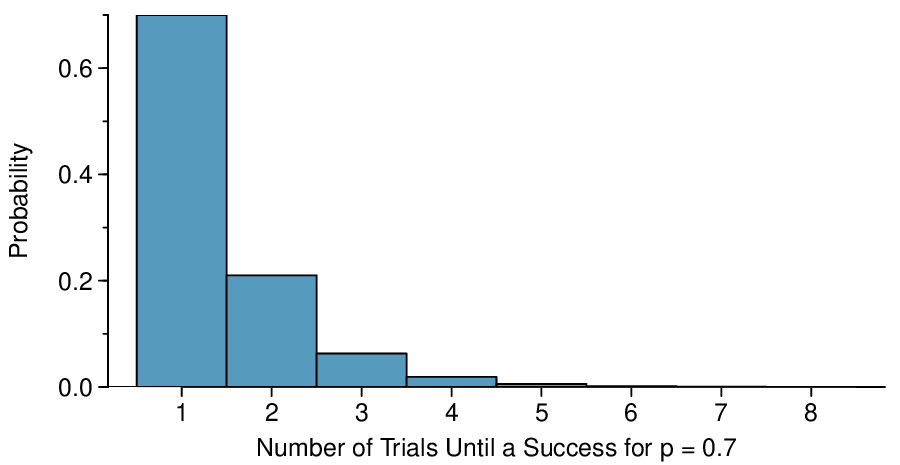
The probability of stopping after the first person is just the chance the first person will not exceed her (or his) deductible: 0.7. The probability the second person is the first to exceed her deductible is
\begin{align*} \amp P(\text{ second person is the first to exceed deductible } )\\ \amp = P(\text{ the first won't, the second will } ) = (0.7)(0.3) = 0.21 \end{align*}
Likewise, the probability it will be the third case is \((0.3)(0.3)(0.7) = 0.063\text{.}\)
If the first success is on the \(x^{th}\) person, then there are \(x-1\) failures and finally 1 success, which corresponds to the probability \((0.7)^{x-1}(0.7)\text{.}\) This is the same as \((1-0.7)^{x-1}(0.7)\text{.}\)
Example 3.5.1 illustrates what the geometric distribution, which describes the waiting time until a success for independent and identically distributed (iid) Bernoulli random variables. In this case, the independence aspect just means the individuals in the example don’t affect each other, and identical means they each have the same probability of success.
The geometric distribution from Example 3.5.1 is shown in Figure 3.5.2. In general, the probabilities for a geometric distribution decrease exponentially fast.
Figure 3.5.2. The geometric distribution when the probability of success is \(p=0.7\text{.}\)
While this text will not derive the formulas for the mean (expected) number of trials needed to find the first success or the standard deviation or variance of this distribution, we present general formulas for each.

Geometric Distribution.

Let \(X\) have a geometric distribution with one parameter \(p\text{,}\) where \(p\) is the probability of a success in one trial. Then the probability of finding the first success in the \(x^{th}\) trial is given by
\begin{gather*} P(X = x) = (1-p)^{x-1}p \end{gather*}
where \(x=1,2,3,\dots\)
The mean (i.e. expected value) and standard deviation of this wait time are given by
\begin{gather*} \mu_{\scriptscriptstyle{X}} = \frac{1}{p} \qquad \sigma_{\scriptscriptstyle{X}} = \frac{\sqrt{1-p\ }}{p} \end{gather*}
It is no accident that we use the symbol \(\mu\) for both the mean and expected value. The mean and the expected value are one and the same.
It takes, on average, \(1/p\) trials to get a success under the geometric distribution. This mathematical result is consistent with what we would expect intuitively. If the probability of a success is high (e.g. 0.8), then we don’t usually wait very long for a success: \(1/0.8 = 1.25\) trials on average. If the probability of a success is low (e.g. 0.1), then we would expect to view many trials before we see a success: \(1/0.1 = 10\) trials.

Guided Practice 3.5.3.

The probability that a particular case would not exceed their deductible is said to be 0.7. If we were to examine cases until we found one that where the person did not exceed her deductible, how many cases should we expect to check?
 2 
We would expect to see about \(1/0.7 \approx 1.43\) individuals to find the first success.

Example 3.5.4.

What is the chance that we would find the first success within the first 3 cases?
Solution.
This is the chance the first (\(X=1\)), second (\(X=2\)), or third (\(X=3\)) case is the first success, which are three disjoint outcomes. Because the individuals in the sample are randomly sampled from a large population, they are independent. We compute the probability of each case and add the separate results:
\begin{align*} \amp P(X=1, 2, \text{ or } 3)\\ \amp = P(X=1)+P(X=2)+P(X=3)\\ \amp = (0.3)^{1-1}(0.7) + (0.7)^{2-1}(0.3) + (0.3)^{3-1}(0.7)\\ \amp = 0.973 \end{align*}
There is a probability of 0.973 that we would find a successful case within 3 cases.

Guided Practice 3.5.5.

Determine a more clever way to solve Example 3.5.4. Show that you get the same result.
 3 
First find the probability of the complement: \(P(\text{no success in first 3 trials}) = 0.3^3 = 0.027\text{.}\) Next, compute one minus this probability: \(1 - P(\text{no success in first 3 trials})= 1 - 0.027 = 0.973\text{.}\)

Example 3.5.6.

Suppose a car insurer has determined that 88% of its drivers will not exceed their deductible in a given year. If someone at the company were to randomly draw driver files until they found one that had not exceeded their deductible, what is the expected number of drivers the insurance employee must check? What is the standard deviation of the number of driver files that must be drawn?
Solution.
In this example, a success is again when someone will not exceed the insurance deductible, which has probability \(p = 0.88\text{.}\) The expected number of people to be checked is \(1 / p = 1 / 0.88 = 1.14\) and the standard deviation is \(\frac{\sqrt{1-p\ }}{p}=\frac{\sqrt{1-0.88\ }}{0.88} = 0.39\text{.}\)

Guided Practice 3.5.7.

Using the results from Example 3.5.6, \(\mu_{X} = 1.14\) and \(\sigma_{X} = 0.39\text{,}\) would it be appropriate to use the normal model to find what proportion of experiments would end in 3 or fewer trials?
 4 
No. The geometric distribution is always right skewed and can never be well-approximated by the normal model.
The independence assumption is crucial to the geometric distribution’s accurate description of a scenario. Mathematically, we can see that to construct the probability of the success on the \(x^{th}\) trial, we had to use the General Multiplication Rule for independent processes. It is no simple task to generalize the geometric model for dependent trials.

Subsection 3.5.3 Technology: geometric probablities

Get started quickly with a Desmos Geometric Calculator
 5 
www.desmos.com/calculator/t1uhsihoiu
that we’ve put together (visit openintro.org/ahss/desmos
 6 
www.openintro.org/ahss/desmos
).

Subsection 3.5.4 Section summary

  • It is useful to model yes/no, success/failure with the values 1 and 0, respectively. We call the probability of success \(p\)and the probability of failure \(1-p\).
  • When the trials are independent and the value of \(p\) is constant, the probability of finding the first success on the \(x^{th}\) trial is given by \((1-p)^{x-1}p\text{.}\) We can see the reasoning behind this formula as follows: for the first success to happen on the \(x^{th}\) trial, it has to not happen the first \(x-1\) trials (with probability \(1-p\)), and then happen on the \(x^{th}\) trial (with probability \(p\)).
  • When we consider the entire distribution of possible values for the how long until the first success, we get a discrete probability distribution known as the geometric distribution. The geometric distribution describes the waiting time until the first success, when the trials are independent and the probability of success, \(p\text{,}\) is constant. If X has a geometric distribution with parameter \(p\text{,}\) then \(P(X=x)=(1-p)^{x-1}p\text{,}\) where \(x=1,2,3\dots\text{.}\)
  • The geometric distribution is always right skewed and, in fact, has no maximum value. The probabilities, though, decrease exponentially fast.
  • Even though the geometric distribution has an infinite number of values, it has a well-defined mean: \(\mu_{X}=\frac{1}{p}\) and standard deviation: \(\sigma_{X} = \frac{\sqrt{1-p \ }}{p}\text{.}\) If the probability of success is \(\frac{1}{10}\text{,}\) then on average it takes 10 trials until we see the first success.
  • Note that when the trials are not independent, we can modify the geometric formula to find the probability that the first success happens on the \(x^{th}\) trial. Instead of simply raising (\(1-p\)) to the \(x-1\text{,}\) multiply the appropriate conditional probabilities.

Exercises 3.5.5 Exercises

1. Is it Bernoulli?

Determine if each trial can be considered an independent Bernoulli trial for the following situations.
  1. Cards dealt in a hand of poker.
  2. Outcome of each roll of a die.
Solution.
  1. No. The cards are not independent. For example, if the first card is an ace of clubs, that implies the second card cannot be an ace of clubs. Additionally, there are many possible categories, which would need to be simplified.
  2. No. There are six events under consideration. The Bernoulli distribution allows for only two events or categories. Note that rolling a die could be a Bernoulli trial if we simply to two events, e.g. rolling a 6 and not rolling a 6, though specifying such details would be necessary.

2. With and without replacement.

In the following situations assume that half of the specified population is male and the other half is female.
  1. Suppose you’re sampling from a room with 10 people. What is the probability of sampling two females in a row when sampling with replacement? What is the probability when sampling without replacement?
  2. Now suppose you’re sampling from a stadium with 10,000 people. What is the probability of sampling two females in a row when sampling with replacement? What is the probability when sampling without replacement?
  3. We often treat individuals who are sampled from a large population as independent. Using your findings from parts (a) and (b), explain whether or not this assumption is reasonable.

3. Eye color, Part I.

A husband and wife both have brown eyes but carry genes that make it possible for their children to have brown eyes (probability 0.75), blue eyes (0.125), or green eyes (0.125).
  1. What is the probability the first blue-eyed child they have is their third child? Assume that the eye colors of the children are independent of each other.
  2. On average, how many children would such a pair of parents have before having a blue-eyed child? What is the standard deviation of the number of children they would expect to have until the first blue-eyed child?
Solution.
  1. \(0.875^2 \times 0.125 = 0.096\text{.}\)
  2. \(\mu= 8\text{,}\) \(\sigma = 7.48\text{.}\)

4. Defective rate.

A machine that produces a special type of transistor (a component of computers) has a 2% defective rate. The production is considered a random process where each transistor is independent of the others.
  1. What is the probability that the \(10^{th}\) transistor produced is the first with a defect?
  2. What is the probability that the machine produces no defective transistors in a batch of 100?
  3. On average, how many transistors would you expect to be produced before the first with a defect? What is the standard deviation?
  4. Another machine that also produces transistors has a 5% defective rate where each transistor is produced independent of the others. On average how many transistors would you expect to be produced with this machine before the first with a defect? What is the standard deviation?
  5. Based on your answers to parts (c) and (d), how does increasing the probability of an event affect the mean and standard deviation of the wait time until success?

5. Bernoulli, the mean.

Use the probability rules from Section 3.4 to derive the mean of a Bernoulli random variable, i.e. a random variable \(X\) that takes value 1 with probability \(p\) and value 0 with probability \(1 - p\text{.}\) That is, compute the expected value of a generic Bernoulli random variable.
Solution.
If \(p\) is the probability of a success, then the mean of a Bernoulli random variable \(X\) is given by \(\mu = E|X| = P(X = 0) \times 0 + P(X = 1) \times 1 = (1 - p) \times 0 + p \times 1 = 0 + p = p\)

6. Bernoulli, the standard deviation.

Use the probability rules from Section 3.4 to derive the standard deviation of a Bernoulli random variable, i.e. a random variable \(X\) that takes value 1 with probability \(p\) and value 0 with probability \(1 - p\text{.}\) That is, compute the square root of the variance of a generic Bernoulli random variable.
You have attempted of activities on this page.