
Advanced High School Statistics: Third Edition

Section 8.4 Inference for the slope of a regression line

Here we encounter our last confidence interval and hypothesis test procedures, this time for making inferences about the slope of the population regression line. We can use this to answer questions such as the following:
  • Is the unemployment rate a significant linear predictor for the loss of the President’s party in the House of Representatives?
  • On average, how much less in college gift aid do students receive when their parents earn an additional $1000 in income?

Subsection 8.4.1 The role of inference for regression parameters

Previously, we found the equation of the regression line for predicting gift aid from family income at Elmhurst College. The slope, \(b\text{,}\) was equal to \(-0.0431\text{.}\) This is the slope for our sample data. However, the sample was taken from a larger population. We would like to use the slope computed from our sample data to estimate the slope of the population regression line.
The equation for the population regression line can be written as
\begin{gather*} \mu_y = \alpha + \beta x \end{gather*}
Here, \(\alpha\) and \(\beta\) represent two model parameters, namely the \(y\)-intercept and the slope of the true or population regression line. (This use of \(\alpha\) and \(\beta\) have nothing to do with the \(\alpha\) and \(\beta\) we used previously to represent the probability of a Type I Error and Type II Error!) The parameters \(\alpha\) and \(\beta\) are estimated using data. We can look at the equation of the regression line calculated from a particular data set:
\begin{align*} \hat{y} =\amp a + bx \end{align*}
and see that \(a\) and \(b\) are point estimates for \(\alpha\) and \(\beta\text{,}\) respectively. If we plug in the values of \(a\) and \(b\text{,}\) the regression equation for predicting gift aid based on family income is:
\begin{gather*} \hat{y}=24.3193-0.0431x \end{gather*}
The slope of the sample regression line, \(-0.0431\text{,}\) is our best estimate for the slope of the population regression line, but there is variability in this estimate since it is based on a sample. A different sample would produce a somewhat different estimate of the slope. The standard error of the slope tells us the typical variation in the slope of the sample regression line and the typical error in using this slope to estimate the slope of the population regression line.
We would like to construct a 95% confidence interval for \(\beta\text{,}\) the slope of the population regression line. As with means, inference for the slope of a regression line is based on the \(t\)-distribution.

Inference for the slope of a regression line.

Inference for the slope of a regression line is based on the \(t\)-distribution with \(n-2\) degrees of freedom, where \(n\) is the number of paired observations.
Once we verify that conditions for using the \(t\)-distribution are met, we will be able to construct the confidence interval for the slope using a critical value \(t^{\star}\) based on \(n-2\) degrees of freedom. We will use a table of the regression summary to find the point estimate and standard error for the slope.

Subsection 8.4.2 Conditions for the least squares line

Conditions for inference in the context of regression can be more complicated than when dealing with means or proportions.
Inference for parameters of a regression line involves the following assumptions:
Linearity. The true relationship between the two variables follows a linear trend. We check whether this is reasonable by examining whether the data follows a linear trend. If there is a nonlinear trend (e.g. left panel of Figure 8.4.1), an advanced regression method from another book or later course should be applied.
Nearly normal residuals. For each \(x\)-value, the residuals should be nearly normal. When this assumption is found to be unreasonable, it is usually because of outliers or concerns about influential points. An example which suggestions non-normal residuals is shown in the second panel of Figure 8.4.1. If the sample size \(n\ge 30\text{,}\) then this assumption is not necessary.
Constant variability. The variability of points around the true least squares line is constant for all values of \(x\text{.}\) An example of non-constant variability is shown in the third panel of Figure 8.4.1.
Independent. The observations are independent of one other. The observations can be considered independent when they are collected from a random sample or randomized experiment. Be careful of data collected sequentially in what is called a time series. An example of data collected in such a fashion is shown in the fourth panel of Figure 8.4.1.
We see in Figure 8.4.1, that patterns in the residual plots suggest that the assumptions for regression inference are not met in those four examples. In fact, identifying nonlinear trends in the data, outliers, and non-constant variability in the residuals are often easier to detect in a residual plot than in a scatterplot.
We note that the second assumption regarding nearly normal residuals is particularly difficult to assess when the sample size is small. We can make a graph, such as a histogram, of the residuals, but we cannot expect a small data set to be nearly normal. All we can do is to look for excessive skew or outliers. Outliers and influential points in the data can be seen from the residual plot as well as from a histogram of the residuals.
Figure 8.4.1. Four examples showing when the inference methods in this chapter are insufficient to apply to the data. In the left panel, a straight line does not fit the data. In the second panel, there are outliers; two points on the left are relatively distant from the rest of the data, and one of these points is very far away from the line. In the third panel, the variability of the data around the line increases with larger values of \(x\text{.}\) In the last panel, a time series data set is shown, where successive observations are highly correlated.

Conditions for inference on the slope of a regression line.

  1. The data is collected from a random sample or randomized experiment.
  2. The residual plot appears as a random cloud of points and does not have any patterns or significant outliers that would suggest that the linearity, nearly normal residuals, constant variability, or independence assumptions are unreasonable.

Subsection 8.4.3 Constructing a confidence interval for the slope of a regression line

We would like to construct a confidence interval for the slope of the regression line for predicting gift aid based on family income for all freshmen at Elmhurst college.
Do conditions seem to be satisfied? We recall that the 50 freshmen in the sample were randomly chosen, so the observations are independent. Next, we need to look carefully at the scatterplot and the residual plot.

Always check conditions.

Do not blindly apply formulas or rely on regression output; always first look at a scatterplot or a residual plot. If conditions for fitting the regression line are not met, the methods presented here should not be applied.
The scatterplot seems to show a linear trend, which matches the fact that there is no curved trend apparent in the residual plot. Also, the standard deviation of the residuals is mostly constant for different \(x\) values and there are no outliers or influential points. There are no patterns in the residual plot that would suggest that a linear model is not appropriate, so the conditions are reasonably met. We are now ready to calculate the 95% confidence interval.
Figure 8.4.2. Left: Scatterplot of gift aid versus family income for 50 freshmen at Elmhurst college. Right: Residual plot for the model shown in left panel.
Table 8.4.3. Summary of least squares fit for the Elmhurst College data, where we are predicting gift aid by the university based on the family income of students.
Estimate Std. Error t value Pr\((>|t|)\)
(Intercept) 24.3193 1.2915 18.83 0.0000
family_income -0.0431 0.0108 -3.98 0.0002

Example 8.4.4.

Construct a 95% confidence interval for the slope of the regression line for predicting gift aid from family income at Elmhurst college.
Solution.
As usual, the confidence interval will take the form:
\begin{gather*} \text{ point estimate } \pm \text{ critical value } \times SE \text{ of estimate } \end{gather*}
The point estimate for the slope of the population regression line is the slope of the sample regression line: \(-0.0431\text{.}\) The standard error of the slope can be read from the table as 0.0108. Note that we do not need to divide 0.0108 by the square root of \(n\) or do any further calculations on 0.0108; 0.0108 is the \(SE\) of the slope. Note that the value of \(t\) given in the table refers to the test statistic, not to the critical value \(t^{\star}\text{.}\) To find \(t^{\star}\) we can use a \(t\)-table. Here \(n=50\text{,}\) so \(df=50-2=48\text{.}\) Using a \(t\)-table, we round down to row \(df=40\) and we estimate the critical value \(t^{\star}=2.021\) for a 95% confidence level. The confidence interval is calculated as:
\begin{align*} -0.0431 \ \pm \ \amp 2.021\times 0.0108\\ =(-0.06\amp 5, -0.021 ) \end{align*}
Note: \(t^{\star}\) using exactly 48 degrees of freedom is equal to 2.01 and gives the same interval of \((-0.065,\ -0.021)\text{.}\)

Example 8.4.5.

Intepret the confidence interval in context. What can we conclude?
Solution.
We are 95% confident that the slope of the population regression line, the true average change in gift aid for each additional $1000 in family income, is between \(-\$0.065\) thousand dollars and \(-\$0.021\) thousand dollars. That is, we are 95% confident that, on average, when family income is $1000 higher, gift aid is between $21 and $65 lower.
Because the entire interval is negative, we have evidence that the slope of the population regression line is less than 0. In other words, we have evidence that there is a significant negative linear relationship between gift aid and family income.
Figure 8.4.6. Left: Scatterplot of head length versus total length for 104 brushtail possums. Right: Residual plot for the model shown in left panel.

Constructing a confidence interval for the slope of regression line.

To carry out a complete confidence interval procedure to estimate the slope of the population regression line \(\beta\text{,}\)
Identify: Identify the parameter and the confidence level, C%.
  • The parameter will be a slope of the population regression line, e.g. the slope of the population regression line relating air quality index to average rainfall per year for each city in the United States.
Choose: Choose the correct interval procedure and identify it by name.
  • Here we use choose the \(t\)-interval for the slope.
Check: Check conditions for using a \(t\)-interval for the slope.
  1. Independence: Data should come from a random sample or randomized experiment. If sampling without replacement, check that the sample size is less than 10% of the population size.
  2. Linearity: Check that the scatterplot does not show a curved trend and that the residual plot shows no \(\cup\) shape pattern
  3. Constant variability: Use the residual plot to check that the standard deviation of the residuals is constant across all \(x\)-values.
  4. Normality: The population of residuals is nearly normal or the sample size is \(\ge 30\text{.}\) If the sample size is less than 30 check for strong skew or outliers in the sample residuals. If neither is found, then the condition that the population of residuals is nearly normal is considered reasonable
Calculate: Calculate the confidence interval and record it in interval form.
  • \(\text{ point estimate } \ \pm\ t^{\star} \times SE\ \text{ of estimate }\text{,}\) \(df = n - 2\)
    • point estimate: the slope \(b\) of the sample regression line
    • \(SE\) of estimate: \(SE\) of slope (find using computer output)
    • \(t^{\star}\text{:}\) use a \(t\)-distribution with \(df = n-2\) and confidence level C%
    • (,)
Conclude: Interpret the interval and, if applicable, draw a conclusion in context.
  • We are C% confident that the true slope of the regression line, the average change in [y] for each unit increase in [x], is between and . If applicable, draw a conclusion based on whether the interval is entirely above, is entirely below, or contains the value 0.

Example 8.4.7.

The regression summary below shows statistical software output from fitting the least squares regression line for predicting head length from total length for 104 brushtail possums. The scatterplot and residual plot are shown above.
Predictor        Coef        SE Coef   T        P
Constant         42.70979    5.17281   8.257   5.66e-13
total_length      0.57290    0.05933   9.657   4.68e-16

S = 2.595    R-Sq = 47.76%    R-Sq(adj) = 47.25%
Construct a 95% confidence interval for the slope of the regression line. Is there convincing evidence that there is a positive, linear relationship between head length and total length? Use the five step framework to organize your work.
Solution.
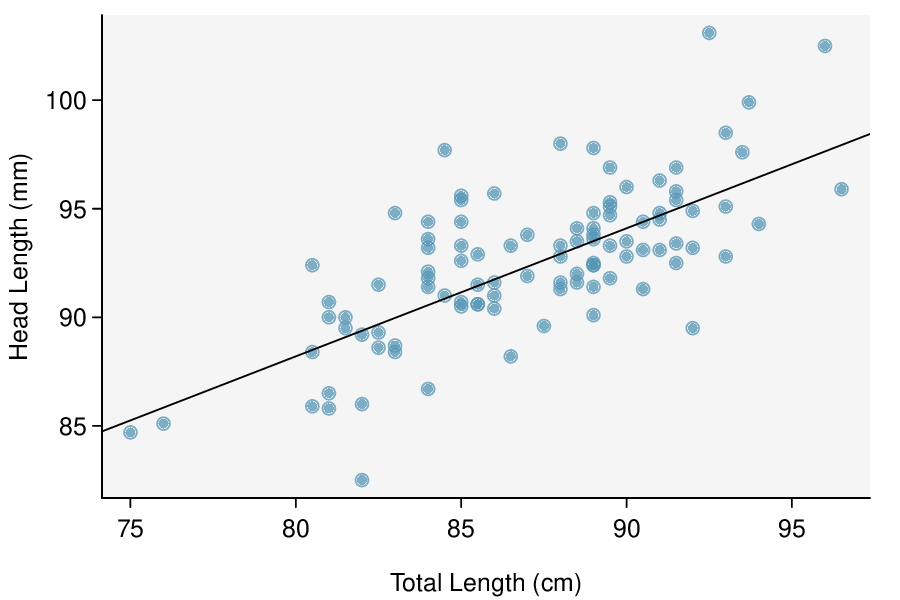
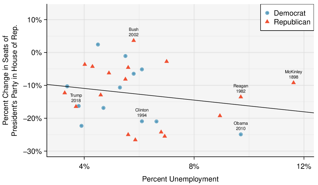
Identify: The parameter of interest is the slope of the population regression line for predicting head length from body length. We want to estimate this at the 95% confidence level.
Choose: Because the parameter to be estimated is the slope of a regression line, we will use the \(t\)-interval for the slope.
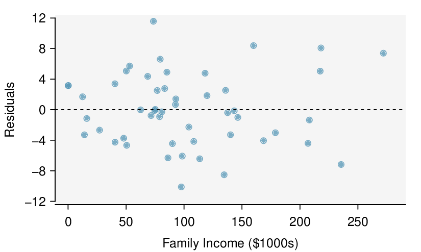
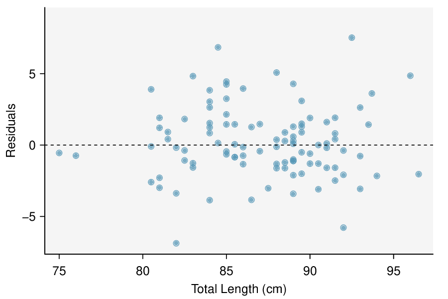
Check: These data come from a random sample. The residual plot shows no pattern so a linear model seems reasonable. The residual plot also shows that the residuals have constant standard deviation. Finally, \(n=104\ge 30\) so we do not have to check for skew in the residuals. All four conditions are met.
Calculate: We will calculate the interval: \(\text{ point estimate } \ \pm\ t^{\star} \times SE\ \text{ of estimate }\)
We read the slope of the sample regression line and the corresponding \(SE\) from the table. The point estimate is \(b = 0.57290\text{.}\) The \(SE\) of the slope is 0.05933, which can be found next to the slope of 0.57290. The degrees of freedom is 
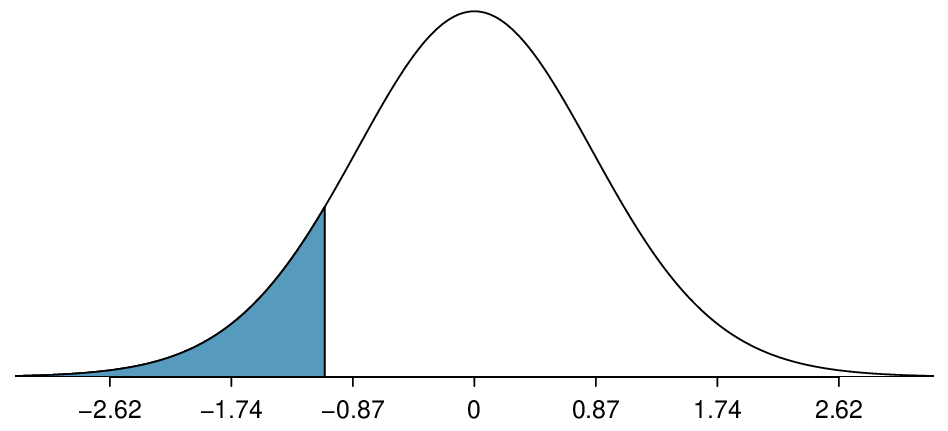
\(df=n-2=104-2=102\text{.}\) As before, we find the critical value \(t^{\star}\) using a \(t\)-table (the \(t^{\star}\) value is not the same as the \(T\)-statistic for the hypothesis test). Using the \(t\)-table at row \(df = 100\) (round down since 102 is not on the table) and confidence level 95%, we get \(t^{\star}=1.984\text{.}\)
So the 95% confidence interval is given by:
\begin{align*} 0.57290 \ \pm\ \amp 1.984\times 0.05933\\ (0.456\amp , 0.691) \end{align*}
Conclude: We are 95% confident that the slope of the population regression line is between 0.456 and 0.691. That is, we are 95% confident that the true average increase in head length for each additional cm in total length is between 0.456mm and 0.691mm. Because the interval is entirely above 0, we do have evidence of a positive linear association between the head length and body length for brushtail possums.

Subsection 8.4.4 Midterm elections and unemployment

Elections for members of the United States House of Representatives occur every two years, coinciding every four years with the U.S. Presidential election. The set of House elections occurring during the middle of a Presidential term are called midterm elections. In America’s two-party system, one political theory suggests the higher the unemployment rate, the worse the President’s party will do in the midterm elections.
To assess the validity of this claim, we can compile historical data and look for a connection. We consider every midterm election from 1898 to 2018, with the exception of those elections during the Great Depression. Figure 8.4.8 shows these data and the least-squares regression line:
\begin{align*} \amp \%\text{ change in House seats for President's party }\\ \amp \qquad \qquad= -7.36 - 0.89\times \text{ (unemployment rate) } \end{align*}
We consider the percent change in the number of seats of the President’s party (e.g. percent change in the number of seats for Republicans in 2018) against the unemployment rate.
Examining the data, there are no clear deviations from linearity, the constant variance condition, or the normality of residuals. While the data are collected sequentially, a separate analysis was used to check for any apparent correlation between successive observations; no such correlation was found.
Figure 8.4.8. The percent change in House seats for the President’s party in each election from 1898 to 2018 plotted against the unemployment rate. The two points for the Great Depression have been removed, and a least squares regression line has been fit to the data. Explore this data set on Tableau Public
 1 
public.tableau.com/profile/openintro#!/vizhome/Chapter8_8/Fig8_248_25
.

Guided Practice 8.4.9.

The data for the Great Depression (1934 and 1938) were removed because the unemployment rate was 21% and 18%, respectively. Do you agree that they should be removed for this investigation? Why or why not?
 2 
We will provide two considerations. Each of these points would have very high leverage on any least-squares regression line, and years with such high unemployment may not help us understand what would happen in other years where the unemployment is only modestly high. On the other hand, these are exceptional cases, and we would be discarding important information if we exclude them from a final analysis.
There is a negative slope in the line shown in Figure 8.4.8. However, this slope (and the y-intercept) are only estimates of the parameter values. We might wonder, is this convincing evidence that the “true” linear model has a negative slope? That is, do the data provide strong evidence that the political theory is accurate? We can frame this investigation as a statistical hypothesis test:
  • \(H_{0}: \beta = 0\text{.}\) The true linear model has slope zero.
  • \(H_{A}: \beta \lt 0\text{.}\) The true linear model has a slope less than zero. The higher the unemployment, the greater the loss for the President’s party in the House of Representatives.
We would reject \(H_0\) in favor of \(H_A\) if the data provide strong evidence that the slope of the population regression line is less than zero. To assess the hypotheses, we identify a standard error for the estimate, compute an appropriate test statistic, and identify the p-value. Before we calculate these quantities, how good are we at visually determining from a scatterplot when a slope is significantly less than or greater than 0? And why do we tend to use a 0.05 significance level as our cutoff? Try out the following activity which will help answer these questions.

Testing for the slope using a cutoff of 0.05.

What does it mean to say that the slope of the population regression line is significantly greater than 0? And why do we tend to use a cutoff of \(\alpha = 0.05\text{?}\) This 5-minute interactive task will explain: www.openintro.org/why05
 3 
www.openintro.org/book/stat/why05/

Subsection 8.4.5 Understanding regression output from software

The residual plot shown in Figure 8.4.10 shows no pattern that would indicate that a linear model is inappropriate. Therefore we can carry out a test on the population slope using the sample slope as our point estimate. Just as for other point estimates we have seen before, we can compute a standard error and test statistic for \(b\text{.}\) The test statistic \(T\) follows a \(t\)-distribution with \(n-2\) degrees of freedom.
Figure 8.4.10. The residual plot shows no pattern that would indicate that a linear model is inappropriate. Explore this data set on Tableau Public
 4 
public.tableau.com/profile/openintro#!/vizhome/Chapter8_8/Fig8_248_25
.

Hypothesis tests on the slope of the regression line.

Use a \(t\)-test with \(n - 2\) degrees of freedom when performing a hypothesis test on the slope of a regression line.
We will rely on statistical software to compute the standard error and leave the explanation of how this standard error is determined to a second or third statistics course. Table 8.4.11 shows software output for the least squares regression line in Figure 8.4.8. The row labeled unemp represents the information for the slope, which is the coefficient of the unemployment variable.
Table 8.4.11. Least squares regression summary for the percent change in seats of president’s party in House of Reprepsentatives based on percent unemployment.
Estimate Std. Error t value Pr\((\gt|t|)\)
(Intercept) -7.3644 5.1553 -1.43 0.1646
unemp -0.8897 0.8350 -1.07 0.2961

Example 8.4.12.

What do the first column of numbers in the regression summary represent?
Solution.
The entries in the first column represent the least squares estimates for the \(y\)-intercept and slope, \(a\) and \(b\) respectively. Using this information, we could write the equation for the least squares regression line as
\begin{gather*} \hat{y} = -7.3644 - 0.8897 x \end{gather*}
where \(y\) in this case represents the percent change in the number of seats for the president’s party, and \(x\) represents the unemployment rate.
We previously used a test statistic \(T\) for hypothesis testing in the context of means. Regression is very similar. Here, the point estimate is \(b=-0.8897\text{.}\) The \(SE\) of the estimate is 0.8350, which is given in the second column, next to the estimate of \(b\text{.}\) This \(SE\) represents the typical error when using the slope of the sample regression line to estimate the slope of the population regression line.
The null value for the slope is 0, so we now have everything we need to compute the test statistic. We have:
\begin{gather*} T = \frac{\text{ point estimate } - \text{ null value } }{SE \text{ of estimate } } = \frac{-0.8897 - 0}{0.8350} = -1.07 \end{gather*}
This value corresponds to the \(T\)-score reported in the regression output in the third column along the unemp row.
Figure 8.4.13. The distribution shown here is the sampling distribution for \(b\text{,}\) if the null hypothesis was true. The shaded tail represents the p-value for the hypothesis test evaluating whether there is convincing evidence that higher unemployment corresponds to a greater loss of House seats for the President’s party during a midterm election.

Example 8.4.14.

In this example, the sample size \(n=27\text{.}\) Identify the degrees of freedom and p-value for the hypothesis test.
Solution.
The degrees of freedom for this test is \(n-2\text{,}\) or \(df = 27-2 = 25\text{.}\) We could use a table or a calculator to find the probability of a value less than -1.07 under the \(t\)-distribution with 25 degrees of freedom. However, the two-side p-value is given in Table 8.4.11, next to the corresponding \(t\)-statistic. Because we have a one-sided alternate hypothesis, we take half of this. The p-value for the test is \(\frac{0.2961}{2}=0.148\text{.}\)
Because the p-value is so large, we do not reject the null hypothesis. That is, the data do not provide convincing evidence that a higher unemployment rate is associated with a larger loss for the President’s party in the House of Representatives in midterm elections.

Don’t carelessly use the p-value from regression output.

The last column in regression output often lists p-values for one particular hypothesis: a two-sided test where the null value is zero. If your test is one-sided and the point estimate is in the direction of \(H_A\text{,}\) then you can halve the software’s p-value to get the one-tail area. If neither of these scenarios match your hypothesis test, be cautious about using the software output to obtain the p-value.

Hypothesis test for the slope of regression line.

To carry out a complete hypothesis test for the claim that there is no linear relationship between two numerical variables, i.e. that \(\beta=0\text{,}\)
Identify: Identify the hypotheses and the significance level, \(\alpha\text{.}\)
  • \(H_0\text{:}\) \(\beta = 0\)
  • \(H_A\text{:}\) \(\beta \ne 0\text{;}\) \(H_A\text{:}\) \(\beta > 0\text{;}\) or \(H_A\text{:}\) \(\beta \lt 0\)
Choose: Choose the correct test procedure and identify it by name.
  • Here we choose the \(t\)-test for the slope.
Check: Check conditions for using a \(t\)-test for the slope.
  1. Independence: Data should come from a random sample or randomized experiment. If sampling without replacement, check that the sample size is less than 10% of the population size.
  2. Linearity: Check that the scatterplot does not show a curved trend and that the residual plot shows no \(\cup\) shape pattern
  3. Constant variability: Use the residual plot to check that the standard deviation of the residuals is constant across all \(x\)-values.
  4. Normality: The population of residuals is nearly normal or the sample size is \(\ge 30\text{.}\) If the sample size is less than 30 check for strong skew or outliers in the sample residuals. If neither is found, then the condition that the population of residuals is nearly normal is considered reasonable
Calculate: Calculate the \(t\)-statistic, \(df\text{,}\) and p-value.
  • \(T= \frac{\text{point estimate} - \text{null value} }{SE \text{ of estimate } }\text{,}\) \(df=n-2\)
    • point estimate: the slope \(b\) of the sample regression line
    • \(SE\) of estimate: \(SE\) of slope (find using computer output)
    • null value: 0
  • p-value = (based on the \(t\)-statistic, the \(df\text{,}\) and the direction of \(H_A\))
Conclude: Compare the p-value to \(\alpha\text{,}\) and draw a conclusion in context.
  • If the p-value is \(\lt \alpha\text{,}\) reject \(H_0\text{;}\) there is sufficient evidence that [\(H_A\) in context].
  • If the p-value is \(> \alpha\text{,}\) do not reject \(H_0\text{;}\) there is not sufficient evidence that [\(H_A\) in context].

Example 8.4.15.

The regression summary below shows statistical software output from fitting the least squares regression line for predicting gift aid based on family income for 50 freshman students at Elmhurst College. The scatterplot and residual plot were shown in Figure 8.4.2.
Predictor        Coef        SE Coef   T        P
Constant         24.31933    1.29145   18.831   < 2e-16
family_income    -0.04307    0.01081   -3.985   0.000229
S = 4.783    R-Sq = 24.86%    R-Sq(adj) = 23.29%
Do these data provide convincing evidence that there is a negative, linear relationship between family income and gift aid? Carry out a complete hypothesis test at the 0.05 significance level. Use the five step framework to organize your work.
Solution.
Identify: We will test the following hypotheses at the \(\alpha=0.05\) significance level.
\(H_0\text{:}\) \(\beta = 0\text{.}\) There is no linear relationship.
\(H_A\text{:}\) \(\beta \lt 0\text{.}\) There is a negative linear relationship.
Here, \(\beta\) is the slope of the population regression line for predicting gift aid from family income at Elmhurst College.
Choose: Because the hypotheses are about the slope of a regression line, we choose the \(t\)-test for a slope.
Check: The data come from a random sample of less than 10% of the total population of freshman students at Elmhurst College. The lack of any pattern in the residual plot indicates that a linear model is reasonable. Also, the residual plot shows that the residuals have constant variance. Finally, \(n=50\ge 30\)). so we do not have to worry too much about any skew in the residuals. All four conditions are met.
Calculate: We will calculate the \(t\)-statistic, degrees of freedom, and the p-value.
\begin{gather*} T = \frac{\text{ point estimate } - \text{ null value } }{SE \text{ of estimate } } \end{gather*}
We read the slope of the sample regression line and the corresponding \(SE\) from the table.
The point estimate is: \(b = -0.04307\text{.}\)
The \(SE\) of the slope is: \(SE = 0.01081\text{.}\)
\begin{gather*} T = \frac{-0.04307 - 0}{0.01081} = -3.985 \end{gather*}
Because \(H_A\) uses a less than sign (\(\lt\)), meaning that it is a lower-tail test, the p-value is the area to the left of \(t=-3.985\) under the \(t\)-distribution with \(50-2=48\) degrees of freedom. The p-value = \(\frac{1}{2}(0.000229)\approx 0.0001\text{.}\)
Conclude: The p-value of 0.0001 is \(\lt 0.05\text{,}\) so we reject \(H_0\text{;}\) there is sufficient evidence that there is a negative linear relationship between family income and gift aid at Elmhurst College.

Guided Practice 8.4.16.

In context, interpret the p-value from the previous example.
 5 
Assuming that the probability model is true and assuming that the null hypothesis is true, i.e. there really is no linear relationship between family income and gift aid at Elmhurst College, there is only a 0.0001 chance of getting a test statistic this small or smaller (\(H_{A}\) uses a <, so the p-value represents the area in the left tail). Because this value is so small, we reject the null hypothesis.

Subsection 8.4.6 Technology: the \(t\)-test for the slope

We generally rely on regression output from statistical software programs to provide us with the necessary quantities: \(b\) and \(SE\) of \(b\text{.}\) However we can also find the test statistic, p-value, and confidence interval using Desmos or a handheld calculator.
Get started quickly with this Desmos T-Test/Interval Calculator
 6 
www.desmos.com/calculator/tbazf5qewp/
(available at openintro.org/ahss/desmos
 7 
openintro.org/ahss/desmos
).
For instructions on implementing the T-Test/Interval on the TI or Casio, see the Graphing Calculator Guides at openintro.org/ahss
 8 
openintro.org/ahss
.

Subsection 8.4.7 Which inference procedure to use for paired data?

In Subsection 7.2.4, we looked at a set of paired data involving the price of textbooks for UCLA courses at the UCLA Bookstore and on Amazon. The left panel of Figure 8.4.17 shows the difference in price (UCLA Bookstore \(-\) Amazon) for each book. Because we have two data points on each textbook, it also makes sense to construct a scatterplot, as seen in the right panel of Figure 8.4.17.
Figure 8.4.17. Left: histogram of the difference (UCLA Bookstore - Amazon) in price for each book sampled. Right: scatterplot of Amazon Price versus UCLA Bookstore price.

Example 8.4.18.

What additional information does the scatterplot provide about the price of textbooks at UCLA Bookstore and on Amazon?
Solution.
With a scatterplot, we see the relationship between the variables. We can see when UCLA Bookstore price is larger, whether Amazon price tends to be larger. We can consider the strength of the correlation and we can plot the linear regression equation.

Example 8.4.19.

Which test should we do if we want to check whether:
  1. prices for textbooks for UCLA courses are higher at the UCLA Bookstore than on Amazon
  2. there is a significant, positive linear relationship between UCLA Bookstore price and Amazon price?
Solution.
In the first case, we are interested in whether the differences (UCLA Bookstore \(-\) Amazon) are, on average, greater than 0, so we would do a 1-sample \(t\)-test for a mean of differences. In the second case, we are interested in whether the slope is significantly greater than 0, so we would do a \(t\)-test for the slope of a regression line.
Likewise, a 1-sample \(t\)-interval for a mean of differences would provide an interval of reasonable values for mean of the differences for all UCLA textbooks, whereas a \(t\)-interval for the slope would provide an interval of reasonable values for the slope of the regression line for all UCLA textbooks.

Inference for paired data.

A matched pairs \(t\)-interval or \(t\)-test for a mean of differences only makes sense when we are asking whether, on average, one variable is greater than another (think histogram of the differences). A \(t\)-interval or \(t\)-test for the slope of a regression line makes sense when we are interested in the linear relationship between them (think scatterplot).

Example 8.4.20.

Previously, we looked at the relationship betweeen body length and head length for bushtail possums. We also looked at the relationship between gift aid and family income for freshmen at Elmhurst College. Could we do a 1-sample \(t\)-test in either of these scenarios?
Solution.
We have to ask ourselves, does it make sense to ask whether, on average, body length is greater than head length? Similarly, does it make sense to ask whether, on average, gift aid is greater than family income? These don’t seem to be meaningful research questions; a 1-sample \(t\)-test for a mean of differences would not be useful here.

Guided Practice 8.4.21.

A teacher gives her class a pretest and a posttest. Does this result in paired data? If so, which hypothesis test should she use?
 9 
Yes, there are two observations for each individual, so there is paired data. The appropriate test depends upon the question she wants to ask. If she is interested in whether, on average, students do better on the posttest than the pretest, should use a 1-sample \(t\)-test for a mean of differences. If she is interested in whether pretest score is a significant linear predictor of posttest score, she should do a \(t\)-test for the slope. In this situation, both tests could be useful, but which one should be used is dependent on the teacher’s research question.

Subsection 8.4.8 Section summary

In Chapter 6, we used a \(\chi^2\) test of independence to test for association between two categorical variables. In this section, we test for association/correlation between two numerical variables.
  • We use the slope \(b\) as a point estimate for the slope \(\beta\) of the population regression line. The slope of the population regression line is the true increase/decrease in \(y\) for each unit increase in \(x\text{.}\) If the slope of the population regression line is 0, there is no linear relationship between the two variables.
  • Under certain assumptions, the sampling distribution of \(b\) is normal and the distribution of the standardized test statistic using the standard error of the slope follows a \(t\)-distribution with \(n-2\) degrees of freedom.
  • When there is \((x, y)\) data and the parameter of interest is the slope of the population regression line, e.g. the slope of the population regression line relating air quality index to average rainfall per year for each city in the United States:
    • Estimate \(\beta\) at the C% confidence level using a \(t\)-interval for the slope.
    • Test \(H_0\text{:}\) \(\beta=0\) at the \(\alpha\) significance level using a \(t\)-test for the slope.
  • The conditions for the \(t\)-interval and \(t\)-test for the slope of a regression line are the same.
    1. Independence: Data should come from a random sample or randomized experiment. If sampling without replacement, check that the sample size is less than 10% of the population size.
    2. Linearity: Check that the scatterplot does not show a curved trend and that the residual plot shows no \(\cup\) shape pattern
    3. Constant variability: Use the residual plot to check that the standard deviation of the residuals is constant across all \(x\)-values.
    4. Normality: The population of residuals is nearly normal or the sample size is \(\ge 30\text{.}\) If the sample size is less than 30 check for strong skew or outliers in the sample residuals. If neither is found, then the condition that the population of residuals is nearly normal is considered reasonable
  • The confidence interval and test statistic are calculated as follows:
    • Confidence interval:  \(\text{ point estimate } \ \pm\ t^{\star} \times SE\ \text{ of estimate }\text{,}\) or
    • Test statistic: \(T = \frac{\text{point estimate} - \text{null value} }{SE\ \text{ of estimate } }\) and p-value
      • point estimate: the slope \(b\) of the sample regression line
      • \(SE\) of estimate: \(SE\) of slope (find using computer output)
      • \(\displaystyle df = n-2\)
  • The confidence interval for the slope of the population regression line estimates the true average increase in the \(y\)-variable for each unit increase in the \(x\)-variable.
  • The \(t\)-test for the slope and the 1-sample \(t\)-test for a mean of differences both involve paired, numerical data. However, the \(t\)-test for the slope asks if the two variables have a linear relationship, specifically if the slope of the population regression line is different from 0. The 1-sample \(t\)-test for a mean of differences, on the other hand, asks if the two variables are in some way the same, specifically if the mean of the population differences is 0.

Exercises 8.4.9 Exercises

1. Body measurements, Part IV.

The scatterplot and least squares summary below show the relationship between weight measured in kilograms and height measured in centimeters of 507 physically active individuals.
Estimate Std. Error t value Pr\((\gt |t|)\)
(Intercept) -105.0113 7.5394 -13.93 0.0000
height 1.0176 0.0440 23.13 0.0000
  1. Describe the relationship between height and weight.
  2. Write the equation of the regression line. Interpret the slope and intercept in context.
  3. Do the data provide strong evidence that an increase in height is associated with an increase in weight? State the null and alternative hypotheses, report the p-value, and state your conclusion.
  4. The correlation coefficient for height and weight is 0.72. Calculate \(R^2\) and interpret it in context.
Solution.
  1. The relationship is positive, moderate-to-strong, and linear. There are a few outliers but no points that appear to be influential.
  2. \(\widehat{\text{weight}} = -105.0113 + 1.0176 \times \text{height}\text{.}\) Slope: For each additional centimeter in height, the model predicts the average weight to be 1.0176 additional kilograms (about 2.2 pounds). Intercept: People who are 0 centimeters tall are expected to weigh -105.0113 kilograms. This is obviously not possible. Here, the \(y\)- intercept serves only to adjust the height of the line and is meaningless by itself.
  3. \(H_{0}:\) The true slope coefficient of height is zero \((\beta = 0)\text{.}\) \(H_{A}:\) The true slope coefficient of height is different than zero \((\beta \ne 0)\text{.}\) The p-value for the two-sided alternative hypothesis \((\beta \ne 0)\) is incredibly small, so we reject \(H_{0}\text{.}\) The data provide convincing evidence that height and weight are positively correlated. The true slope parameter is indeed greater than 0.
  4. \(R^2 = 0.72^2 = 0.52\text{.}\) Approximately 52% of the variability in weight can be explained by the height of individuals.

2. MCU, predict US theater sales..

The Marvel Comic Universe movies were an international movie sensation, containing 23 movies at the time of this writing. Here we consider a model predicting an MCU film’s gross theater sales in the US based on the first weekend sales performance in the US. The data are presented below in both a scatterplot and the model in a regression table. Scientific notation is used below, e.g. 42.5e6 corresponds to \(42.5 \times 10^{6}\text{.}\)
Estimate Std. Error t value Pr\((\gt|t|)\)
(Intercept) 42.5e6 26.6e6 1.6 0.1251
opening weekend US 2.4361 0.1739 14.01 0.0000
  1. Describe the relationship between gross theater sales in the US and first weekend sales in the US.
  2. Write the equation of the regression line. Interpret the slope and intercept in context.
  3. Do the data provide strong evidence that higher opening weekend sale is associated with higher gross theater sales? State the null and alternative hypotheses, report the p-value, and state your conclusion.
  4. The correlation coefficient for gross sales and first weekend sales is 0.950. Calculate \(R^{2}\) and interpret it in context.
  5. Suppose we consider a set of all films ever released. Do you think the relationship between opening weekend sales and total sales would have as strong of a relationship as what we see with the MCU films?

3. Spouses, Part II.

The scatterplot below summarizes womens’ heights and their spouses’ heights for a random sample of 170 married women in Britain, where both partners’ ages are below 65 years. Summary output of the least squares fit for predicting spouse’s height from the woman’s height is also provided in the table.
Estimate Std. Error t value Pr\((\gt|t|)\)
(Intercept) 43.5755 4.6842 9.30 0.0000
height_spouse 0.2863 0.0686 4.17 0.0000
  1. Is there strong evidence in this sample that taller women have taller spouses? State the hypotheses and include any information used to conduct the test.
  2. Write the equation of the regression line for predicting the height of a woman’s spouse based on the woman’s height.
  3. Interpret the slope and intercept in the context of the application.
  4. Given that \(R^2 = 0.09\text{,}\) what is the correlation of heights in this data set?
  5. You meet a married woman from Britain who is 5’9" (69 inches). What would you predict her spouse’s height to be? How reliable is this prediction?
  6. You meet another married woman from Britain who is 6’7" (79 inches). Would it be wise to use the same linear model to predict her spouse’s height? Why or why not?
Solution.
  1. \(H_{0}: \beta = 0\text{;}\) \(H_{A}: \beta \ne 0\text{.}\) The p-value, as reported in the table, is incredibly small and is smaller than 0.05, so we reject \(H_{0}\text{.}\) The data provide convincing evidence that womens’ and spouses’ heights are positively correlated.
  2. \(\widehat{\text{height}_{S}} = 43.5755 + 0.2863 \times \text{height}_{W}\text{.}\)
  3. Slope: For each additional inch in woman’s height, the spouse’s height is expected to be an additional 0.2863 inches, on average. Intercept: Women who are 0 inches tall are predicted to have spouses who are 43.5755 inches tall. The intercept here is meaningless, and it serves only to adjust the height of the line.
  4. The slope is positive, so \(r\) must also be positive. \(r= \sqrt{0.09} = 0.30\)
  5. 63.2612. Since \(R^2\) is low, the prediction based on this regression model is not very reliable.
  6. No, we should avoid extrapolating.

4. Urban homeowners, Part II.

Exercise 8.2.10.13 gives a scatterplot displaying the relationship between the percent of families that own their home and the percent of the population living in urban areas. Below is a similar scatterplot, excluding District of Columbia, as well as the residuals plot. There were 51 cases.
  1. For these data, \(R^2 = 0.28\text{.}\) What is the correlation? How can you tell if it is positive or negative?
  2. Examine the residual plot. What do you observe? Is a simple least squares fit appropriate for these data?

5. Murders and poverty, Part II.

Exercise 8.2.10.9 presents regression output from a model for predicting annual murders per million from percentage living in poverty based on a random sample of 20 metropolitan areas. The model output is also provided below.
Estimate Std. Error t value Pr\((\gt|t|)\)
(Intercept) -29.901 7.789 -3.839 0.001
poverty% 2.559 0.390 6.562 0.000
\(s = 5.512\) \(R^2 = 70.52\%\) \(R^2_{adj} = 68.89\%\)
  1. What are the hypotheses for evaluating whether poverty percentage is a significant predictor of murder rate?
  2. State the conclusion of the hypothesis test from part (a) in context of the data.
  3. Calculate a 95% confidence interval for the slope of poverty percentage, and interpret it in context of the data.
  4. Do your results from the hypothesis test and the confidence interval agree? Explain.
Solution.
  1. \(H_{0}: \beta = 0\text{;}\) \(H_{A}: \beta \ne 0\)
  2. The p-value for this test is approximately 0, therefore we reject \(H_{0}\text{.}\) The data provide convincing evidence that poverty percentage is a significant predictor of murder rate.
  3. \(n = 20\text{;}\) \(df = 18\text{;}\) \(T^{*}_{18} = 2.10\text{;}\) \(2.559 \pm 2.10 \times 0.390 = (1.74, 3.378)\text{;}\) For each percentage point poverty is higher, murder rate is expected to be higher on average by 1.74 to 3.378 per million.
  4. Yes, we rejected \(H_{0}\) and the confidence interval does not include 0.

6. Babies.

Is the gestational age (time between conception and birth) of a low birth-weight baby useful in predicting head circumference at birth? Twenty-five low birth-weight babies were studied at a Harvard teaching hospital; the investigators calculated the regression of head circumference (measured in centimeters) against gestational age (measured in weeks). The estimated regression line is
\begin{gather*} \widehat{\text{head circumference}} = 3.91 + 0.78 \times \text{gestational age} \end{gather*}
  1. What is the predicted head circumference for a baby whose gestational age is 28 weeks?
  2. The standard error for the coefficient of gestational age is 0.35, which is associated with \(df=23\text{.}\) Does the model provide strong evidence that gestational age is significantly associated with head circumference?

Subsection 8.4.10 Chapter Highlights

This chapter focused on describing the linear association between two numerical variables and fitting a linear model.
  • The correlation coefficient, \(r\text{,}\) measures the strength and direction of the linear association between two variables. However, \(r\) alone cannot tell us whether data follow a linear trend or whether a linear model is appropriate.
  • The explained variance, \(R^2\text{,}\) measures the proportion of variation in the \(y\) values explained by a given model. Like \(r\text{,}\) \(R^2\) alone cannot tell us whether data follow a linear trend or whether a linear model is appropriate.
  • Every analysis should begin with graphing the data using a scatterplot in order to see the association and any deviations from the trend (outliers or influential values). A residual plot helps us better see patterns in the data.
  • When the data show a linear trend, we fit a least squares regression line of the form: \(\hat{y} = a+bx\text{,}\) where \(a\) is the \(y\)-intercept and \(b\) is the slope. It is important to be able to calculate \(a\) and \(b\) using the summary statistics and to interpret them in the context of the data.
  • A residual, \(y-\hat{y}\text{,}\) measures the error for an individual point. The standard deviation of the residuals, \(s\text{,}\) measures the typical size of the residuals.
  • \(\hat{y} = a+bx\) provides the best fit line for the observed data. To estimate or hypothesize about the slope of the population regression line, first confirm that the residual plot has no pattern and that a linear model is reasonable, then use a \(t\)-interval for the slope or a \(t\)-test for the slope with \(n-2\) degrees of freedom.
In this chapter we focused on simple linear models with one explanatory variable. More complex methods of prediction, such as multiple regression (more than one explanatory variable) and nonlinear regression can be studied in a future course.
You have attempted of activities on this page.