Objectives: Learning objectives
-
Explain the logic of hypothesis testing, including setting up hypotheses and drawing a conclusion based on the set significance level and the calculated p-value.
-
Set up the null and alternative hypothesis in words and in terms of population parameters.
-
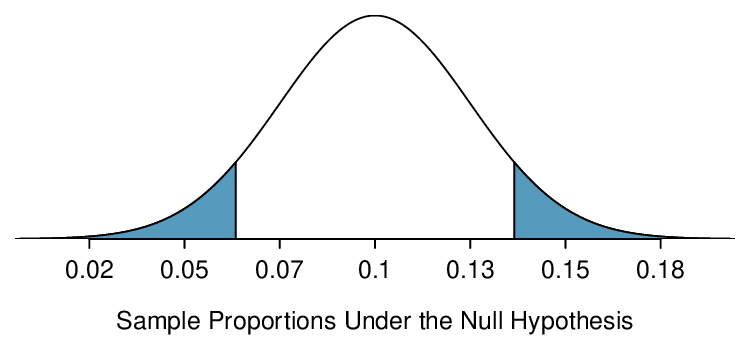
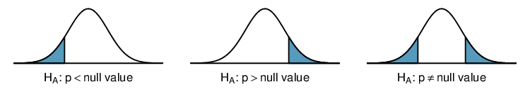
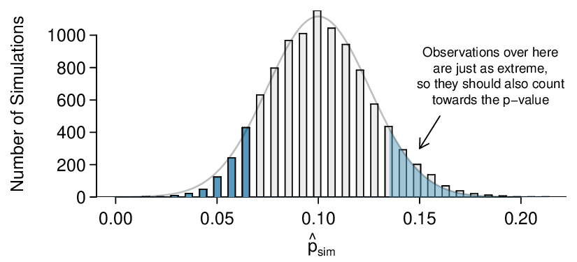
Interpret a p-value in context and recognize how the calculation of the p-value depends upon the direction of the alternative hypothesis.
-
Define and interpret the concept statistically significant.
-
Interpret Type I, Type II Error, and power in the context of hypothesis testing.
-
Distinguish between statistically significant and practically significant, and recognize the role that sample size plays here.
-
Understand the two general conditions for when the confidence interval and hypothesis testing procedures apply and explain why these conditions are necessary.