
Advanced High School Statistics: Third Edition

Section 4.3 Sampling distribution for a difference

In this section, we consider the case where instead of having one random sample from a population of interest, we have two independent random samples and we are interested in how far the sample values might be from one another. We describe the sampling distribution for the difference of sample proportions and the difference of sample means, and we find the probability that the difference would be greater than or less than a certain amount.

Subsection 4.3.1 The mean and SD for a difference of two random variables (review)

In Section 3.4, we saw how to find the mean and standard deviation of a difference of two random variables \(X\) and \(Y\text{.}\) We found that:
\begin{gather*} E(X-Y)=E(X)-E(Y) \end{gather*}
That is, if we have the mean of each random variable, \(\mu_{X}\) and \(\mu_{Y}\text{,}\) then the mean of the difference of the random variables is simply the differences of the individual means. This should seem very straightforward.
The situation is a little more complex when looking at the variability of the difference of \(X\) and \(Y\) . Here we’re going to require a condition be met, specifically that \(X\) and \(Y\) are independent random variables. When that independence condition is met, then the following formula for the standard deviation of the difference, \(X-Y\text{,}\) holds:
\begin{gather*} SD(X-Y) = \sqrt{(SD(X))^{2}+(SD(Y))^{2}} \end{gather*}
These two formulas from probability play an important role in applications where we look at the difference of two sample proportions \((\hat{p}_{1}-\hat{p}_{2})\) or the difference of sample means \((\bar{x}_{1}-\bar{x}_{2})\text{.}\)

Subsection 4.3.2 Differenece of Sample Proportions

In Section 4.1 we considered a county where the proportion of people with blood type O+ is known to be 35%, and we described the distribution of the sample statistic \(\hat{p}\) from a random sample of size \(n\) from this population.
Let us now consider two counties. In County 1, it is known that 35% of people have blood type O+. In County 2, it is known that 30% of people have blood type O+. If we take a random sample of size 50 from County 1 and a random sample of size 50 from County 2, what is the probability that we will get a higher proportion with blood type O+ in the County 2 sample?
We know that the expected proportion with blood type O+ is lower in County 2. However, due to random variability, there is still some chance that the sample from County 2 will have a higher proportion with blood type O+. First, we need to find the mean (expected value) and the standard deviation for the difference of sample proportions \(\hat{p}_{1}-\hat{p}_{2}\text{.}\) For this, we use the two formulas from Subsection 4.3.1 in the context of the difference of sample proportions by substituting \(X=\hat{p}_{1}\) and \(Y=\hat{p}_{2}\text{.}\)
\begin{gather*} E(\hat{p}_{1}-\hat{p}_{2}) = E(\hat{p}_{1})-E(\hat{p}_{2})= p_{1}-p_{2}\\ SD(\hat{p}_{1}-\hat{p}_{2}) = \sqrt{(SD(\hat{p}_{1}))^{2}+(SD(\hat{p}_{2}))^{2}}=\sqrt{\frac{p_{1}(1-p_{1})}{n_{1}}+\frac{p_{2}(1-p_{2})}{n_{2}}} \end{gather*}
That is, given two independent random samples, the distribution of all possible values of \(\hat{p}_{1}-\hat{p}_{2}\) is centered on the true difference \(p_{1}-p_{2}\) and the typical distance or error of \(\hat{p}_{1}-\hat{p}_{2}\) from \(p_{1}-p_{2}\) is given by \(\sqrt{\frac{p_{1}(1-p_{1})}{n_{1}}+\frac{p_{2}(1-p_{2})}{n_{2}}}\text{.}\) Using \(\mu\) for mean and \(\sigma\) for SD, we summarize this as follows

Mean and standard deviation of a difference of sample proportions.

The mean and standard deviation of the difference of sample proportions describe the center and spread of the distribution of all possible differences \(\hat{p}_{1}-\hat{p}_{2}\text{.}\) Given population proportions \(p_{1}\) and \(p_{2}\) and random samples of size \(n_{1}\) and \(n_{2}\) where the independence condition is satisfied, we have the following.
\begin{align*} \mu_{\hat{p}_{1}-\hat{p}_{2}}=p_{1}-p_{2} \amp \amp \sigma_{\hat{p}_{1}-\hat{p}_{2}}=\sqrt{\frac{p_{1}(1-p_{1})}{n_{1}}+\frac{p_{2}(1-p_{2})}{n_{2}}} \end{align*}
As we saw previously, the independence condition is satisfied if the data is collected from an experiment with two randomly assigned treatments or collected from 2 independent random samples, where each sample size is less than 10% of the population size if done without replacement.
Having described the center and spread of the distribution of the difference of sample proportions, we need to understand the shape of the distribution. When looking at the sum or difference of random variables, if each variable is nearly normal, then the sum and difference are also nearly normal. This property will be very useful, as it says that when each sample proportion has a nearly normal distribution, then the difference of sample proportions will also be nearly normal, and we can use normal approximation to estimate probabilities that the difference will be greater or less than some value.

Example 4.3.1.

Let’s return to the blood type example. In County 1, it is known that 35% of people have blood type O+. In County 2, it is known that 30% of people have blood type O+. If we take a random sample of size 50 from County 1 and a random sample of size 50 from County 2, what is the probability that we will get a higher proportion with blood type O+ in the County 2 sample?
Solution.
We want to find \(P(\hat{p}_{1} \lt \hat{p}_{2})\text{,}\) This is equivalent to \(P(\hat{p}_{1}-\hat{p}_{2} \lt 0)\text{.}\)
Let us first determine whether the independence condition is satisfied and whether normal approximation will be appropriate. We have two random samples, and the samples are independent of each other as they are from distinct populations. It is reasonable to assume that each sample size is less than 10% of the county population size. We now check the success-failure condition for each group.
\begin{align*} n_{1}p_{1} = 50 \times 0.35 = 17.5 \ge 10 \amp n_{1}(1-p_{1}) = 50 \times (1-0.35) = 32.5 \ge 10\\ n_{2}p_{2} = 50 \times 0.30 = 15.0 \ge 10 \amp n_{2}(1-p_{2}) = 50 \times (1-0.30) = 35.0 \ge 10 \end{align*}
The independence condition is satisfied and the success-failure condition is met for both groups, so the distribution of \(\hat{p}_{1}-\hat{p}_{2}\) can be said to be nearly normal.
We now find the mean and the standard deviation of \(\hat{p}_{1}-\hat{p}_{2}\text{.}\)
\begin{gather*} \mu_{\hat{p}_{1}-\hat{p}_{2}}=p_{1}-p_{2} = 0.35-0.30 = 0.05\\ \sigma_{\hat{p}_{1}-\hat{p}_{2}}= \sqrt{\frac{p_{1}(1-p_{1})}{n_{1}}+\frac{p_{2}(1-p_{2})}{n_{2}}} = \sqrt{\frac{0.35(1-0.35)}{50}+\frac{0.30(1-0.30)}{50}} = 0.0935 \end{gather*}
Recall, we want to find \(P(\hat{p}_{1}-\hat{p}_{2} \lt 0)\text{.}\) We use the calculated mean and standard deviation of \(\hat{p}_{1}-\hat{p}_{2}\) to find a Z-score for the value of interest, which is 0.
\begin{gather*} Z=\frac{x-\mu}{\sigma} = \frac{0-0.05}{0.0935}= -0.535 \end{gather*}
Using technology to find the area to the left of -0.535 under the standard normal curve, we obtain \(P(\hat{p}_{1}-\hat{p}_{2}) \approx P(Z \lt −0.535) = 0.296\text{.}\) Even though County 2 has a lower proportion of people with blood type O+, with these small sample sizes, there is still a 29.6% chance that the sample from County 2 ends up with a higher proportion with blood type O+ than the sample from County 1.

Subsection 4.3.3 Difference of sample means

In Section 4.2 we started with all of the data from the 2017 Cherry Blossom Run, and we considered what the sampling distribution for a mean would look like for random samples of size \(n\text{.}\)
The population mean for all the runners is 94.52 minutes and the population standard deviationis 8.97 minutes. Imagine taking two independent random samples of size 50 from this population. We know that the sampling distribution for the mean would have the same center and spread in each sample, but what about the sampling distribution for the difference of the sample means? What is the likelihood that the sample means from these two independent random samples would differ by more than 3 minutes?
To answer this, we consider two scenarios. First, consider the possibility that the mean of sample 1 is more than 3 minutes greater than the mean of sample 2. That is, we want to find \(P(\bar{x}_{1}-\bar{x}_{2}) \gt 3\text{.}\) Second, it is also possible that the mean of sample 2 is more than 3 minutes greater than the mean of sample 1, so we also need to find \(P(\bar{x}_{2}-\bar{x}_{1}) \gt 3\text{,}\) which we could also write as \(P(\bar{x}_{1}-\bar{x}_{2}) \lt -3\text{.}\) We now see that we are interested in the upper and lower tail of the distribution of \(\bar{x}_{1}-\bar{x}_{2}\text{.}\) As we will soon see, the distribution of \(\bar{x}_{1}-\bar{x}_{2}\) follows a normal distribution when certain conditions are met, and in those cases we can find one tail and then double it thanks to the symmetry of the normal distribution.
Let’s find the mean (expected value) and the standard deviation for the difference of sample means, \(\bar{x}_{1}-\bar{x}_{2}\text{.}\) We again use the formulas discussed in Subsection 4.3.1 for the difference in two independent random normal variables, \(X − Y\text{,}\) but this time we substitute in \(X=\bar{x}_{1}\) and \(Y=\bar{x}_{2}\text{:}\)
\begin{gather*} E(\bar{x}_{1}-\bar{x}_{2}) = E(\bar{x}_{1})-E(\bar{x}_{2})= \mu_{1}-\mu_{2}\\ SD(\bar{x}_{1}-\bar{x}_{2}) = \sqrt{(SD(\bar{x}_{1}))^{2}+(SD(\bar{x}_{1}))^{2}}=\sqrt{\frac{\sigma_{1}^2}{n_{1}}+\frac{\sigma_{2}^2}{n_{2}}} \end{gather*}
That is, given two independent random samples, the distribution of all possible values of \(\bar{x}_{1}-\bar{x}_{2}\) is centered on the true difference \(\mu_{1}-\mu_{2}\) and the typical distance or error of \(\bar{x}_{1}-\bar{x}_{2}\) from \(\mu_{1}-\mu_{2}\) is given by \(\sqrt{\frac{\sigma_{1}^2}{n_{1}}+\frac{\sigma_{2}^2}{n_{2}}}\)

Mean and standard deviation of a difference of sample means.

The mean and standard deviation of the difference of sample means describe the center and spread of the distribution of all possible differences \(\bar{x}_{1}-\bar{x}_{2}\text{.}\) Given population means \(\mu_{1}\) and \(\mu_{2}\text{,}\) individual population standard deviations \(\sigma_{1}\) and \(\sigma_{2}\text{,}\) and two random samples of size \(n_{1}\) and \(n_{2}\text{,}\) then if the independence condition is satisfied, we have the following:
\begin{align*} \mu_{\bar{x}_{1}-\bar{x}_{2}} = \mu_{1}-\mu_{2} \amp \amp \sigma_{\bar{x}_{1}-\bar{x}_{2}} = \sqrt{\frac{\sigma_{1}^2}{n_{1}}+\frac{\sigma_{2}^2}{n_{2}}} \end{align*}
Recall that in Subsection 4.3.2, we also noted that the sum or difference of random variables will also nearly normal, if each variable is itself nearly normal and the two random variables are also independent of each other. We will frequently use this principle to determine when the difference of sample means can be modeled using a normal distribution.

Example 4.3.2.

Lett’s return to the Cherry Blossom Run application. We have that the population mean for all the runners in the 2017 Cherry Blossom Run is 94.52 minutes and the population standard deviation is 8.97 minutes. If we take two independent random samples of 50 runners, what is the probability that the sample means from these two samples will differ by more than 3 minutes?
Solution.
We want to find \(P(\bar{x}_{1}-\bar{x}_{2} \gt 3) + P(\bar{x}_{1}-\bar{x}_{2} \lt -3)\text{.}\)
Let us first determine whether the independence condition is satisfied and whether normal approximation will be appropriate. We have two random samples, and the samples are distinct and independent of each other. The sample sizes are each less than 10% of total population of runners. Also, because the sample sizes n1 and n2 are both 50, and \(50 \ge 30\text{,}\) we don’t need the distribution of all run times to be nearly normal. With these conditions met, we have shown that the distribution of \(\bar{x}_{1}-\bar{x}_{2}\) is nearly normal.
\begin{gather*} \mu_{\bar{x}_{1}-\bar{x}_{2}} = \mu_{1}-\mu_{2} = 94.52 - 94.52 = 0\\ \sigma_{\bar{x}_{1}-\bar{x}_{2}} = \sqrt{\frac{\sigma_{1}^2}{n_{1}}+\frac{\sigma_{2}^2}{n_{2}}} = \sqrt{\frac{8.97^2}{50}+\frac{8.97^2}{50}} =1.79 \end{gather*}
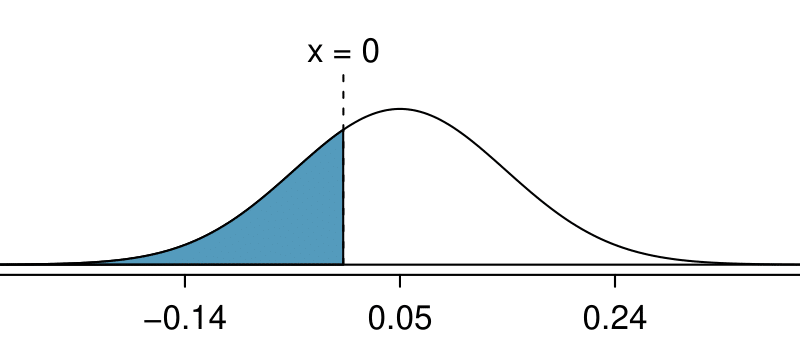
To find \(P(\bar{x}_{1}-\bar{x}_{2} \gt 3)\text{,}\) we use the calculated mean and standard deviation of \(\bar{x}_{1}-\bar{x}_{2}\) to first find a Z-score for the difference of interest, which is 3.
\begin{gather*} Z=\frac{x-\mu}{\sigma} = \frac{3-0}{1.79} = 1.676 \end{gather*}
Using technology, to find the area to the right of 1.676 under the standard normal curve, we have: 
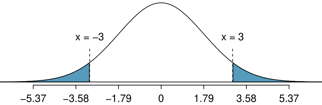
\(P(\bar{x}_{1}-\bar{x}_{2} \gt 3) \approx P(Z \gt 1.676) = 0.047\text{.}\) Because the normal distribution of interest is centered at zero, the \(P(\bar{x}_{1}-\bar{x}_{2} \lt -33)\) tail area will have the same size. So to get the total of the two tail areas, we double 0.047. Even though the samples are from the same population of runners, there is still a \(2 \times 0.047 = 0.094\) probability, or a 9.4% chance, that the sample means will differ by more than 3 minutes.

Subsection 4.3.4 Section Summary

  • When two random variables each follow a nearly normal distribution, the distribution of their difference also follows a nearly normal distribution.
  • Both \(\hat{p}_{1}-\hat{p}_{2}\) and \(\bar{x}_{1}-\bar{x}_{2}\) are statistics that can take on different values from one random sample to the next. As such, they have sampling distributions that can be described by their center, spread, and shape.
  • Three important facts about the sampling distribution for the difference of sample proportions \(\hat{p}_{1}-\hat{p}_{2}\) where the observations can be treated as independent:
    • The mean of the difference of sample proportions, denoted by \(\mu_{\hat{p}_{1}-\hat{p}_{2}}\text{,}\) is equal to \(p_{1}-p_{2}\text{.}\) (center)
    • The SD of the difference of sample proportions, denoted by \(\sigma_{\hat{p}_{1}-\hat{p}_{2}}\text{,}\) is equal to \(\sqrt{\frac{p_{1}(1-p_{1})}{n_{1}}+\frac{p_{2}(1-p_{2})}{n_{2}}}\text{.}\) (spread)
    • When both groups meet the success-failure condition, the difference of sample proportions can be modeled using a normal distribution. (shape)
  • Three important facts about the sampling distribution for the difference of sample means \(\bar{x}_{1}-\bar{x}_{2}\) where the observations can be treated as independent:
    • The mean of the difference of sample means, denoted by \(\mu_{\bar{x}_{1}-\bar{x}_{2}}\text{,}\) is equal to \(\mu_{1}-\mu_{2}\text{.}\) (center)
    • The SD of the difference of sample means, denoted by \(\sigma_{\bar{x}_{1}-\bar{x}_{2}}\) is equal to \(\sqrt{\frac{\sigma_{1}^2}{n_{1}}+\frac{\sigma_{2}^2}{n_{2}}}\text{.}\) (spread)
    • When both populations are nearly normal or when \(n_{1} \ge 30\) and \(n_{2} \ge 30\text{,}\) the difference of sample means can be modeled using a normal distribution. (shape)
  • When the difference of sample proportions \(\hat{p}_{1}-\hat{p}_{2}\) or the difference of sample means \(\bar{x}_{1}-\bar{x}_{2}\) follow a nearly normal distribution, we can find the probability that the difference is greater than or less than a certain amount by finding a Z-score and using the normal approximation.

Exercises 4.3.5 Exercises

1. Difference of proportions, Part 1.

The fraction of workers who are considered “supercommuters”, because they commute more than 90 minutes to get to work, varies by state. Suppose the following were the exact values for Nebraska and New York:
Table 4.3.3.
State Proportion Supercommuters
Nebraska 0.01
New York 0.06
Now suppose that we plan a study to survey 1000 people from each state, and we will compute the sample proportions \(\hat{p}_{NE}\) for Nebraska and \(\hat{p}_{NY}\) for New York.
  1. What is the associated mean and standard deviation of \(\hat{p}_{NE}\text{?}\)
  2. What is the associated mean and standard deviation of \(\hat{p}_{NY}\text{?}\)
  3. Calculate and interpret the mean and standard deviation associated with the difference in sample proportions for the two groups, \(\hat{p}_{NE}-\hat{p}_{NY}\text{.}\)
  4. How are the standard deviations from parts (a), (b), and (c) related?
Solution.
  1. \(mu_{\hat{p}_{NE}= 0.01}\text{.}\) \(\sigma_{\hat{p}_{NE}}=0.0031\text{.}\)
  2. \(mu_{\hat{p}_{NY}=0.06}\text{.}\) \(\sigma_{\hat{p}_{NY}}=0.0075\text{.}\)
  3. \(mu_{\hat{p}_{NY}-\hat{p}_{NE}}=0.06-0.01\text{.}\) \(\sigma_{\hat{p}_{NY}-\hat{p}_{NE}}=0.0081\text{.}\)
  4. We can think of \(\hat{p}_{NE}\) and \(\hat{p}_{NY}\) as being random variables, and we are considering the standard deviation of the difference of these two random variables, so we square each standard deviation, add them together, and then take the square root of the sum:
    \begin{gather*} SD_{\hat{p}_{NY}-\hat{p}_{NE}}= \sqrt{SD_{\hat{p}_{NY}}^2+SD_{\hat{p}_{NE}}^2} \end{gather*}

2. Difference of proportions, Part 2.

The fraction of workers who are considered “supercommuters”, because they commute more than 90 minutes to get to work, varies by state. Suppose the following were the exact values for Nebraska and New York:
Table 4.3.4.
State Proportion Supercommuters
Nebraska 0.01
New York 0.06
Now suppose that we plan a study to survey 1000 people from each state, and we will compute the sample proportions \(\hat{p}_{NE}\) for Nebraska and \(\hat{p}_{NY}\) for New York.
  1. What distribution is associated with the difference \(\hat{p}_{NE}-\hat{p}_{NY}\text{?}\) Justify your answer.
  2. Determine the probability that \(\hat{p}_{NE}-\hat{p}_{NY}\) will be larger than 0.055.
  3. Determine the probability that \(\hat{p}_{NE}-\hat{p}_{NY}\) will be smaller than 0.4.

3. Difference of means, Part 1.

Suppose we will collect two random samples from the following distribution:
Table 4.3.5.
Mean Standard Deviation Sample Size
Sample 1 15 20 50
Sample 2 20 10 30
In each of the parts below, consider the sample means \(\bar{x}_{1}\) and \(\bar{x}_{2}\) that we might observe from these two samples.
  1. What is the associated mean and standard deviation of \(\bar{x}_{1}\text{?}\)
  2. What is the associated mean and standard deviation of \(\bar{x}_{2}\text{?}\)
  3. Calculate and interpret the mean and standard deviation associated with the difference in sample means for the two groups, \(\bar{x}_{2}-\bar{x}_{1}\text{.}\)
  4. How are the standard deviations from parts (a), (b), and (c) related?
Solution.
  1. \(\mu_{\bar{x}_{1}} = 15\text{.}\) \(\sigma_{\bar{x}_{1}} = 20/ \sqrt{50}=2.8284\text{.}\)
  2. \(\mu_{\bar{x}_{2}} =20\text{.}\) \(\sigma_{\bar{x}_{2}} = 10/ \sqrt{30}=1.8257\text{.}\)
  3. \(\mu_{\bar{x}_{2}-\bar{x}_{1}}=20-15=5\text{.}\) \(\sigma_{\bar{x}_{2}-\bar{x}_{1}} =sqrt{(20/ \sqrt{50})^2+(10/ \sqrt{30})^2}=3.3665\)
  4. Think of \(\bar{x}_{1}\) and \(\bar{x}_{2}\) as being random variables, and we are considering the standard deviation of the difference of these two random variables, so we square each standard deviation, add them together, and then take the square root of the sum:
    \begin{gather*} SD_{\bar{x}_{2}-\bar{x}_{1}}= \sqrt{SD_{\bar{x}_{2}}^2+SD_{\bar{x}_{1}}^2} \end{gather*}

4. Difference of means, Part 2.

Suppose we will collect two random samples from the following distribution:
Table 4.3.6.
Mean Standard Deviation Sample Size
Sample 1 15 20 50
Sample 2 20 10 30
In each of the parts below, consider the sample means \(\bar{x}_{1}\) and \(\bar{x}_{2}\) that we might observe from these two samples.
  1. What distribution is associated with the difference \(\bar{x}_{2}-\bar{x}_{1}\text{?}\) Justify your answer.
  2. Determine the probability that \(\bar{x}_{2}-\bar{x}_{1}\) will be larger than 7.
  3. Determine the probability that \(\bar{x}_{2}-\bar{x}_{1}\) will be smaller than 3.
  4. Determine the probability that \(\bar{x}_{2}-\bar{x}_{1}\) will be smaller than 0.

Subsection 4.3.6 Chapter Highlights

This chapter began by introducing the idea of a sampling distribution. As with any distribution, we can summarize a sampling distribution with regard to its center, spread, and shape. A common thread that ran through this chapter is the application of normal approximation (introduced in Section 2.3.) to different sampling distributions.
The key steps are included for each of the normal approximation scenarios below. To verify that observations can be considered independent, verify that you have one of the following: a random process, a random sample with replacement, or a random sample without replacement of less than 10% of the population. To satisfy the independence condition when working with two groups, we require 2 independent random samples with replacement, 2 independent samples without replacement of less than 10% of their populations, or an experiment with 2 randomly assigned treatments. For completion and comparison purposes, we include cases introduced in earlier chapters as well in the overview below.
  1. Normal approximation for numerical data: (introduced in Section 2.3).
    • Verify that observations can be treated as independent and that population is approximately normal.
    • Use a normal model with mean \(\mu\) and SD \(\sigma\text{.}\)
  2. Normal approximation for a sample proportion (with categorical data):
    • Verify that observations can be treated as independent and that \(np \ge 10\) and \(n(1-p) \ge 10\text{.}\)
    • Use a normal model with mean \(\mu_{\hat{p}}=p\) and SD \(\sigma_{\hat{p}}= \sqrt{\frac{p(1-p)}{n}}\text{.}\)
  3. Normal approximation for a sample mean (with numerical data):
    • Verify that observations can be treated as independent and that population is approximately normal or that \(n \ge 30\text{.}\)
    • Use a normal model with mean \(\mu_{\bar{x}}=\mu\) and SD \(\sigma_{\bar{x}}= \frac{\sigma}{\sqrt{n}}\)
  4. Normal approximation for a difference of sample proportions:
    • Verify that observations can be treated as independent and that \(n_{1}p_{1} \ge 10\text{,}\) \(n_{1}(1-p_{1}) \ge 10\text{,}\) \(n_{2}p_{2} \ge 10\text{,}\) and \(n_{2}(1-p_{2}) \ge 10\text{.}\)
    • Use a normal model with mean \(\mu_{\hat{p}_{1}-\hat{p}_{2}} =p_{1}-p_{2} \) and \(\sigma_{\hat{p}_{1}-\hat{p}_{2}}=\sqrt{\frac{p_{1}(1-p_{1})}{n_{1}}+\frac{p_{2}(1-p_{2})}{n_{2}}}\)
  5. Normal approximation for a difference of sample means:
    • Verify that observations can be treated as independent and that both populations are nearly normal or both \(n_{1}\) and \(n_{2}\) are \(\ge 30\text{.}\)
    • Use a normal model with mean: \(\mu_{\bar{x}_{1}-\bar{x}_{2}} = \mu_{1}-\mu{2}\) and SD \(\sigma_{\bar{x}_{1}-\bar{x}_{2}} = \sqrt{\frac{\sigma_{1}^2}{n_{1}}+\frac{\sigma_{2}^2}{n_{2}}}\text{.}\)
Cases 1, 3 and 5 are for numerical variables, while cases 2 and 4 are for categorical yes/no variables.
In the case of proportions and counts, we never look to see if the population is normal. That would not make sense because a yes/no variable cannot have a normal distribution.
The Central Limit Theorem is the mathematical rule that ensures that when the sample size is sufficiently large, the sample mean/sum and sample proportion/count will be approximately normal.
You have attempted of activities on this page.