Advanced High School Statistics: Third Edition

Section 7.4 Chapter exercises

Exercises Exercises

1. Gaming and distracted eating, Part I.

A group of researchers are interested in the possible effects of distracting stimuli during eating, such as an increase or decrease in the amount of food consumption. To test this hypothesis, they monitored food intake for a group of 44 patients who were randomized into two equal groups. The treatment group ate lunch while playing solitaire, and the control group ate lunch without any added distractions. Patients in the treatment group ate 52.1 grams of biscuits, with a standard deviation of 45.1 grams, and patients in the control group ate 27.1 grams of biscuits, with a standard deviation of 26.4 grams. Do these data provide convincing evidence that the average food intake (measured in amount of biscuits consumed) is different for the patients in the treatment group? Assume that conditions for inference are satisfied.
 1 
R.E. Oldham-Cooper et al. “Playing a computer game during lunch affects fullness, memory for lunch, and later snack intake”. In: The American Journal of Clinical Nutrition 93.2 (2011), p. 308.
Solution.
\(H_{0} : \mu_{T} = \mu_{C}\text{.}\) \(H_{A} : \mu_{T} \ne \mu_{C}\text{.}\) \(T = 2.24\text{,}\) \(df = 21 \rightarrow \text{p-value } = 0.036\text{.}\) Since \(\text{p-value } < 0.05\text{,}\) reject \(H_{0}\text{.}\) The data provide strong evidence that the average food consumption by the patients in the treatment and control groups are different. Furthermore, the data indicate patients in the distracted eating (treatment) group consume more food than patients in the control group.
2. Gaming and distracted eating, Part II.

The researchers from Exercise 7.4.1 also investigated the effects of being distracted by a game on how much people eat. The 22 patients in the treatment group who ate their lunch while playing solitaire were asked to do a serial-order recall of the food lunch items they ate. The average number of items recalled by the patients in this group was 4. 9, with a standard deviation of 1.8. The average number of items recalled by the patients in the control group (no distraction) was 6.1, with a standard deviation of 1.8. Do these data provide strong evidence that the average number of food items recalled by the patients in the treatment and control groups are different?

3. Sample size and pairing.

Determine if the following statement is true or false, and if false, explain your reasoning: If comparing means of two groups with equal sample sizes, always use a paired test.
Solution.
False. While it is true that paired analysis requires equal sample sizes, only having the equal sample sizes isn’t, on its own, sufficient for doing a paired test. Paired tests require that there be a special correspondence between each pair of observations in the two groups.

4. College credits.

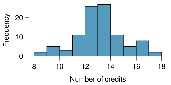
A college counselor is interested in estimating how many credits a student typically enrolls in each semester. The counselor decides to randomly sample 100 students by using the registrar’s database of students. The histogram below shows the distribution of the number of credits taken by these students. Sample statistics for this distribution are also provided.
Min 8
Q1 13
Median 14
Mean 13.65
SD 1.91
Q3 15
Max 18
  1. What is the point estimate for the average number of credits taken per semester by students at this college? What about the median?
  2. What is the point estimate for the standard deviation of the number of credits taken per semester by students at this college? What about the IQR?
  3. Is a load of 16 credits unusually high for this college? What about 18 credits? Explain your reasoning.
  4. The college counselor takes another random sample of 100 students and this time finds a sample mean of 14.02 units. Should she be surprised that this sample statistic is slightly different than the one from the original sample? Explain your reasoning.
  5. The sample means given above are point estimates for the mean number of credits taken by all students at that college. What measures do we use to quantify the variability of this estimate? Compute this quantity using the data from the original sample.

5. Hen eggs.

The distribution of the number of eggs laid by a certain species of hen during their breeding period has a mean of 35 eggs with a standard deviation of 18.2. Suppose a group of researchers randomly samples 45 hens of this species, counts the number of eggs laid during their breeding period, and records the sample mean. They repeat this 1,000 times, and build a distribution of sample means.
  1. What is this distribution called?
  2. Would you expect the shape of this distribution to be symmetric, right skewed, or left skewed? Explain your reasoning.
  3. Calculate the variability of this distribution and state the appropriate term used to refer to this value.
  4. Suppose the researchers’ budget is reduced and they are only able to collect random samples of 10 hens. The sample mean of the number of eggs is recorded, and we repeat this 1,000 times, and build a new distribution of sample means. How will the variability of this new distribution compare to the variability of the original distribution?
Solution.
  1. We are building a distribution of sample statistics, in this case the sample mean. Such a distribution is called a sampling distribution.
  2. Because we are dealing with the distribution of sample means, we need to check to see if the Central Limit Theorem applies. Our sample size is greater than 30, and we are told that random sampling is employed. With these conditions met, we expect that the distribution of the sample mean will be nearly normal and therefore symmetric.
  3. Because we are dealing with a sampling distribution, we measure its variability with the standard error. \(SE = 18.2/ \sqrt{45} = 2.713\)
  4. The sample means will be more variable with the smaller sample size.

6. Forest management.

Forest rangers wanted to better understand the rate of growth for younger trees in the park. They took measurements of a random sample of 50 young trees in 2009 and again measured those same trees in 2019. The data below summarize their measurements, where the heights are in feet:
2009 2010 Differences
\(\bar{x}\) 12.0 24.5 12.5
\(s\) 3.5 9.5 7.2
\(n\) 50 50 50
Construct a 99% confidence interval for the average growth of (what had been) younger trees in the park over 2009-2019.

7. Exclusive relationships.

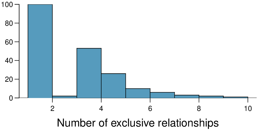
A survey conducted on a reasonably random sample of 203 undergraduates asked, among many other questions, about the number of exclusive relationships these students have been in. The histogram below shows the distribution of the data from this sample. The sample average is 3.2 with a standard deviation of 1.97.
Estimate the average number of exclusive relationships Duke students have been in using a 90% confidence interval and interpret this interval in context. Check any conditions required for inference, and note any assumptions you must make as you proceed with your calculations and conclusions.
Solution.
Independence: it is a random sample, so we can assume that the students in this sample are independent of each other with respect to number of exclusive relationships they have been in. Notice that there are no students who have had no exclu-sive relationships in the sample, which suggests some student responses are likely missing (perhaps only positive values were reported). The sample size is at least 30, and there are no particularly extreme outliers, so the normality condition is reasonable. 90% CI: \((2.97, 3.43)\text{.}\) We are 90% confident that undergraduate students have been in 2.97 to 3.43 exclusive relationships, on average.

8. Age at first marriage, Part I.

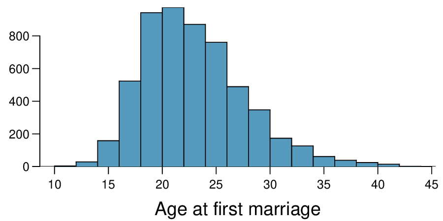
The National Survey of Family Growth conducted by the Centers for Disease Control gathers information on family life, marriage and divorce, pregnancy, infertility, use of contraception, and men’s and women’s health. One of the variables collected on this survey is the age at first marriage. The histogram below shows the distribution of ages at first marriage of 5,534 randomly sampled women between 2006 and 2010. The average age at first marriage among these women is 23.44 with a standard deviation of 4.72.
 2 
Centers for Disease Control and Prevention, National Survey of Family Growth, 2010.
Estimate the average age at first marriage of women using a 95% confidence interval, and interpret this interval in context. Discuss any relevant assumptions.

9. Online communication.

A study suggests that the average college student spends 10 hours per week communicating with others online. You believe that this is an underestimate and decide to collect your own sample for a hypothesis test. You randomly sample 60 students from your dorm and find that on average they spent 13.5 hours a week communicating with others online. A friend of yours, who offers to help you with the hypothesis test, comes up with the following set of hypotheses. Indicate any errors you see.
\begin{gather*} H_{0}:\bar{x}\lt 10 \text{ hours}\\ H_{A}:\bar{x}\gt 13.5 \text{ hours} \end{gather*}
Solution.
First, the hypotheses should be about the population mean (\(\mu\)), not the sample mean. Second, the null hypothesis should have an equal sign and the alternative hypothesis should be about the null hypothesized value, not the observed sample mean. The correct way to set up these hypotheses is shown below:
\begin{gather*} H_{0}: \mu = 10 \text{hours}\\ H_{A}: \mu \ne 10 \text{hours} \end{gather*}
A two-sided test allows us to consider the possibility that the data show us something that we would find surprising.

10. Age at first marriage, Part II.

Exercise 7.4.8 presents the results of a 2006 - 2010 survey showing that the average age of women at first marriage is 23.44. Suppose a social scientist thinks this value has changed since the survey was taken. Below is how she set up her hypotheses. Indicate any errors you see.
\begin{gather*} H_{0}:\bar{x}\neq 23.44 \text{ years old}\\ H_{A}:\bar{x} = 23.44 \text{ years old} \end{gather*}

11. Friday the 13th, Part I.

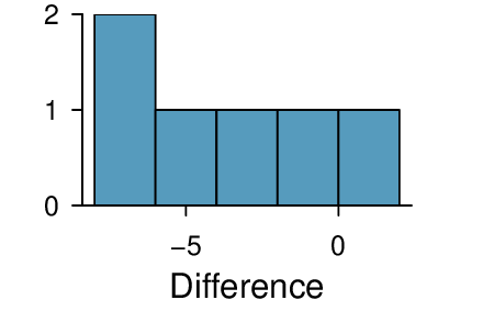
In the early 1990’s, researchers in the UK collected data on traffic flow, number of shoppers, and traffic accident related emergency room admissions on Friday the \(13^{th}\) and the previous Friday, Friday the \(6^{th}\text{.}\) The histograms below show the distribution of number of cars passing by a specific intersection on Friday the \(6^{th}\) and Friday the \(13^{th}\) for many such date pairs. Also given are some sample statistics, where the difference is the number of cars on the 6th minus the number of cars on the 13th.
 3 
T.J. Scanlon et al. “Is Friday the 13th Bad For Your Health?” In: BMJ 307 (1993), pp. 1584-1586.
\(6^{th}\) \(13^{th}\) Diff.
\(\bar{x}\) 128,385 126,550 1,835
\(s\) 7,259 7,664 1,176
\(n\) 10 10 10
  1. Are there any underlying structures in these data that should be considered in an analysis? Explain.
  2. What are the hypotheses for evaluating whether the number of people out on Friday the \(6^{th}\) is different than the number out on Friday the \(13^{th}\text{?}\)
  3. Check conditions to carry out the hypothesis test from part (b).
  4. Calculate the test statistic and the p-value.
  5. What is the conclusion of the hypothesis test?
  6. Interpret the p-value in this context.
  7. What type of error might have been made in the conclusion of your test? Explain.
Solution.
  1. These data are paired. For example, the Friday the 13th in say, September 1991, would probably be more similar to the Friday the 6th in September 1991 than to Friday the 6th in another month or year.
  2. Let \(\mu_{diff} = \mu_{sixth} - \mu_{thirteenth}\text{.}\) \(H_{0} : \mu_{diff} = 0\text{.}\) \(H_{A} : \mu_{diff} \ne 0\text{.}\)
  3. Independence: The months selected are not random. However, if we think these dates are roughly equivalent to a simple random sample of all such Friday 6th/13th date pairs, then independence is reasonable. To proceed, we must make this strong assumption, though we should note this assumption in any reported results. Normality: With fewer than 10 observations, we would need to see clear outliers to be concerned. There is a borderline outlier on the right of the histogram of the differences, so we would want to report this in formal analysis results.
  4. \(T = 4.93\) for \(df = 10 - 1 = 9 \rightarrow \text{p-value } = 0.001\text{.}\)
  5. Since \(\text{p-value } \lt 0.05\text{,}\) reject \(H_{0}\text{.}\) The data provide strong evidence that the average number of cars at the intersection is higher on Friday the \(6^{th}\) than on Friday the \(13^{th}\text{.}\) (We should exercise caution about generalizing the interpretation to all intersections or roads.)
  6. If the average number of cars passing the intersection actually was the same on Friday the \(6^{th}\) and \(13^{th}\text{,}\) then the probability that we would observe a test statistic so far from zero is less than 0.01.
  7. We might have made a Type 1 Error, i.e. incorrectly rejected the null hypothesis.

12. Friday the 13th, Part II.

The Friday the 13\(^{th}\) study reported in Exercise 7.4.11 also provides data on traffic accident related emergency room admissions. The distributions of these counts from Friday the 6\(^{th}\) and Friday the 13\(^{th}\) are shown below for six such paired dates along with summary statistics. You may assume that conditions for inference are met.
6\(^{th}\) 13\(^{th}\) diff
Mean 7.5 10.83 -3.33
SD 3.33 3.6 3.01
n 6 6 6
  1. Conduct a hypothesis test to evaluate if there is a difference between the average numbers of traffic accident related emergency room admissions between Friday the 6\(^{th}\) and Friday the 13\(^{th}\text{.}\)
  2. Calculate a 95% confidence interval for the difference between the average numbers of traffic accident related emergency room admissions between Friday the 6\(^{th}\) and Friday the 13\(^{th}\text{.}\)
  3. The conclusion of the original study states, “Friday 13th is unlucky for some. The risk of hospital admission as a result of a transport accident may be increased by as much as 52%. Staying at home is recommended.” Do you agree with this statement? Explain your reasoning.
You have attempted of activities on this page.