Inference for a single proportion

Section 6.1 Inference for a single proportion

In this section, we will apply the inferential procedures introduced in Chapter 5 to the context of a single proportion, and we will explore how to do sample size calculations for data collection purposes. We will answer questions such as the following:

Do greater than half of adults in the U.S. oppose nuclear energy?
🔗

🔗
What percent of adults in the U.S. approve of the way the Supreme Court is handling its job?
🔗

🔗
What is the standard error is associated with this estimate?
🔗

🔗
How do we construct a confidence interval for this value?
🔗

🔗
What sample size is required to estimate this within a 3% margin of error using a 95% confidence level?
🔗

🔗

🔗

Objectives: Learning objectives

State and verify whether or not the conditions for inference on a proportion using a normal distribution are met.
🔗

🔗
Recognize that the success-failure condition and the standard error calculation are different for the test and for the confidence interval and explain why this is the case.
🔗

🔗
Carry out a complete hypothesis test and confidence interval procedure for a single proportion.
🔗

🔗
Find the minimum sample size needed to estimate a proportion with C% confidence and a margin of error no greater than a certain value.
🔗

🔗
Recognize that margin of error calculations only measure sampling error, and that other types of errors may be present.
🔗

🔗

🔗

Subsection 6.1.1 Distribution of a sample proportion (review)

The distribution of a sample proportion, such as the distribution of all possible values for the proportion of people who share a particular opinion in a poll, was introduced in Section 4.1. When the sampling distribution of a sample proportion,

\hat{p},

is approximately normal, we can use confidence intervals and hypothesis tests based on a normal distribution. We call these Z-intervals and Z-tests for short. Here, we review the conditions necessary for a sample proportion to be modeled using a normal distribution.

🔗

Conditions for the sampling distribution of $\hat{p}$ being nearly normal.

The sampling distribution of a sample proportion,

\hat{p},

based on a random sample of size

n

from a population with a true proportion

p,

is nearly normal when

the sample observations are independent and
🔗

🔗
$n p \geq 10$ and $n (1 - p) \geq 10 .$ This is called the success-failure condition.
🔗

🔗

🔗

If these conditions are met, then the sampling distribution of

\hat{p}

is nearly normal with mean

μ_{\hat{p}} = p

and standard deviation

σ_{\hat{p}} = \sqrt{\frac{p (1 - p)}{n}} .

🔗

Subsection 6.1.2 Checking conditions for inference using a normal distribution

We can use a normal model for inference for a proportion when the sampling distribution for the sample proportion is nearly normal. We check that this assumption is reasonable by assessing the independence assumption and verifying that the success-failure condition is met.

🔗

Independent. Observations can be considered independent when the data are collected from a random process, such as tossing a coin, or from a random sample. Without a random sample or process, the standard error formula would not apply, and it is unclear to what population the inference would apply. When sampling without replacement from a finite population, the observations can be considered independent when sampling less than 10% of the population.
¹
When sampling without replacement and sampling greater than 10% of the population, a modified standard error formula should be used.
🔗

🔗
Nearly normal sampling distribution. We saw in Section 4.1 that the sampling distribution of a sample proportion will be nearly normal when the success-failure condition is met, i.e. when the expected number of success and failures are both at least 10.
🔗

🔗

🔗

In our examples, we generally sample from large populations, such as the United States. In these cases, we do not explicitly verify that the sample size is less than 10% of the population size. However, in borderline cases, one should remember to check this condition as well to ensure that the standard error estimate is reasonable.

🔗

Subsection 6.1.3 Confidence intervals for a proportion

🔗

The Gallup organization began measuring the public’s view of the Supreme Court’s job performance in 2000, and has measured it every year since then with the question: “Do you approve or disapprove of the way the Supreme Court is handling its job?”. In 2018, the Gallup poll randomly sampled 1,033 adults in the U.S. and found that 53% of them approved.

https://news.gallup.com/poll/237269/supreme-court-approval-highest-2009.aspx

We know that 53% is just a point estimate. What range of values are reasonable estimates for the percent of the population that approved of the job the Supreme Court is doing? We can use the confidence interval procedure introduced in the previous chapter to answer this question, but first we must clearly identify the parameter we’re trying to estimate and be sure that a Z-interval will be appropriate. The following examples walk through the various steps for carrying out a confidence interval procedure using the Gallup poll data.

🔗

Example 6.1.1.

Identify the population of interest and the parameter of interest for the Gallup poll about the U.S. Supreme Court.

🔗

Solution.

Gallup sampled from U.S. adults, therefore the population of interest, and the population to which we can make an inference, is U.S. adults. We know the percent of the sample that said they approve of the job the Supreme Court is doing. However, we do not know what percent of the population would approve. The parameter of interest, which is unknown, is the percent of all U.S. adults that approve of the job the Supreme Court is doing. This is the quantity that we seek to estimate with the confidence interval.

🔗

Example 6.1.2.

Can the sample proportion

\hat{p}

be modeled using a normal distribution?

🔗

Solution.

In order to construct a Z-interval, the sample statistic must be able to be modeled using a normal distribution. Gallup took a random sample, so the first condition (the independence condition) is satisfied. We must also test the second condition (the success-failure condition) to ensure that the sample size is large enough for the central limit theorem to apply. The success-failure condition is met when

n p

and

n (1 - p)

are at least 10. Since

p

is always unknown when constructing a confidence interval for

p,

we use the sample proportion

\hat{p}

to check this condition. Here we have:

\begin{matrix} n \hat{p} = 1033 (0.53) = 547 (“successes”) \\ n (1 - \hat{p}) = 1033 (1 - 0.53) = 486 (“failures”) \end{matrix}

🔗

The second condition is satisfied since 547 and 486 are both at least 10. With the two conditions satisfied, we can model the sample proportion

\hat{p}

using a normal model and we can construct a Z-interval.

🔗

Example 6.1.3.

Calculate the point estimate and the

S E

of the estimate.

🔗

Solution.

The point estimate for the unknown parameter

p

(the proportion of all U.S. adults) who approve of the job the Supreme Court is doing) is the sample proportion. The point estimate here is

\hat{p} = 0.53 .

🔗

Because the point estimate is the sample proportion, the

S E

of the estimate is the

S E

\hat{p} .

In Section 4.1, we learned that the formula for the standard deviation of

\hat{p}

\begin{matrix} σ_{\hat{p}} = \sqrt{\frac{p (1 - p)}{n}} \end{matrix}

🔗

The proportion

p

is unknown, so we use the sample proportion

\hat{p}

to find the

S E

\hat{p} .

\begin{matrix} S E = \sqrt{\frac{\hat{p} (1 - \hat{p})}{n}} \end{matrix}

🔗

Here

\hat{p} = 0.53

and

n = 1, 033,

so the

S E

of the sample proportion is:

\begin{matrix} S E = \sqrt{\frac{0.53 (1 - 0.53)}{1033}} = 0.016 \end{matrix}

🔗

Example 6.1.4.

Construct a 90% confidence interval for

p,

the proportion of all U.S. adults that approve of the job the Supreme Court is doing.

🔗

Solution.

Recall that the general form of a confidence interval is:

\begin{matrix} point estimate \pm critical value \times S E of estimate \end{matrix}

🔗

We have already found the point estimate and the

S E

of the estimate. Because we previously verified that

\hat{p}

can be modeled using a normal distribution, the critical value is a

z^{⋆} .

The

z^{⋆}

value can be found in the

t

-table in Section B.3, using the bottom row (

\infty

), where the column corresponds to the confidence level. Here the confidence level is 90%, so

z^{⋆}

=1.65. We can now construct the 90% confidence interval as follows.

\begin{aligned} point estimate \pm & z^{⋆} \times S E of estimate \\ 0.53 \pm & 1.65 \times 0.016 \\ = (0.504, 0.556) \end{aligned}

🔗

We are 90% confident that the true proportion of U.S. adults who approve of the job the Supreme Court is doing is between 0.504 and 0.556.

🔗

Example 6.1.5.

Based on the interval, is there evidence that more than half of U.S. adults approve of the job the Supreme Court is doing?

🔗

Solution.

The 90% confidence interval (0.504, 0.556) provides an interval of reasonable values for the parameter. The value 0.50 is not in the interval, therefore can be considered unreasonable. Because the entire interval is above 0.50, we do have evidence, at the 90% confidence level, that more than half of U.S. adults (at the time of this poll) approve of the job the Supreme Court is doing.

🔗

Example 6.1.6.

Do we have evidence at the 95% confidence level that more than half of U.S. adults approve of the job the Supreme Court is doing?

🔗

Solution.

First, we observe that a 95% confidence interval will be wider than a 90% confidence interval. For a 95% Z-interval,

z^{⋆} = 1.96 .

The 95% confidence interval is:

\begin{aligned} 0.53 \pm 1.96 \times 0.016 \\ = (0.499, 0.561) \end{aligned}

🔗

Now, we see that 0.50 is just barely inside the interval, making it within the range of reasonable values. Therefore, we do not have evidence, at the 95% confidence level, that more than half of U.S. adults (at the time of this poll) approve of the job the Supreme Court is doing.

🔗

Notice that we come to a different conclusion based on different confidence levels, which may feel a little jarring. However, this will happen with real data, and it highlights why it is important to be explicit in identifying the confidence level being used.

🔗

Having worked through this example, we now summarize the steps for constructing a confidence interval for a proportion using the five step framework introduce in Chapter 5.

🔗

Constructing a confidence interval for a proportion.

To carry out a complete confidence interval procedure to estimate a single proportion

p,

🔗

Identify: Identify the parameter and the confidence level, C%.

The parameter will be a population proportion, e.g. the proportion of all U.S. adults that approve of the job the Supreme Court is doing.
🔗

🔗

🔗

Choose: Choose the correct interval procedure and identify it by name.

Here we choose the 1-proportion Z-interval.
🔗

🔗

🔗

Check: Check conditions for the sampling distribution of

\hat{p}

to be nearly normal.

Data come from a random sample or random process.
🔗

🔗
$n \hat{p} \geq 10$ and $n (1 - \hat{p}) \geq 10$ (Make sure to plug in numbers.)
🔗

🔗

🔗

Calculate: Calculate the confidence interval and record it in interval form.

🔗

$point estimate \pm z^{⋆} \times S E of estimate$
🔗
- point estimate: the sample proportion $\hat{p}$
  🔗
  
  🔗
- $S E$ of estimate: $\sqrt{\frac{\hat{p} (1 - \hat{p})}{n}}$
  🔗
  
  🔗
- $z^{⋆} :$ use a $t$ -table at row $\infty$ and confidence level C
  🔗
  
  🔗
🔗
🔗
(,)
🔗

🔗

🔗

Conclude: Interpret the interval and, if applicable, draw a conclusion in context.

We are C% confident that the true proportion of [...] is between and . If applicable, draw a conclusion based on whether the interval is entirely above, is entirely below, or contains the value of interest.
🔗

🔗

🔗

Example 6.1.7.

A February 2018 Marist Poll reports: “Many Americans (68%) think there is intelligent life on other planets.” The results were based on a random sample of 1,033 adults in the U.S. Does this poll provide evidence at the 95% confidence level that greater than half of all U.S. adults think there is intelligent life on other planets? Carry out a confidence interval procedure to answer this question. Use the five step framework to organize your work.

🔗

Solution.

Identify: First we identify the parameter of interest. Here the parameter is the true proportion of U.S. adults that think there is intelligent life on other planets. We will estimate this at the 95% confidence level.

🔗

Choose: Because the parameter to be estimated is a single proportion, we will use a 1-proportion Z-interval.

🔗

Check: We must check that a Z-interval is appropriate, meaning that the sample proportion can be modeled using a normal distribution. The problem states that the data come from a random sample. Also, we must check the success-failure condition. Here, we have that

1033 (0.68) \geq 10

and

1033 (1 - 0.68) \geq 10 .

Both conditions are met so we can proceed with a 1-proportion Z-interval.

🔗

Calculate: We will calculate the interval:

\begin{matrix} point estimate \pm z^{⋆} \times S E of estimate \end{matrix}

🔗

The point estimate is the sample proportion:

\hat{p} = 0.68

🔗

The

S E

of the sample proportion is:

\sqrt{\frac{\hat{p} (1 - \hat{p})}{n}} = \sqrt{\frac{0.68 (1 - 0.68)}{1033}} = 0.015 .

🔗

z^{⋆}

is found using the

t

-table at row

\infty

and confidence level C%.

🔗

For a 95% confidence level,

z^{⋆}

= 1.96.

🔗

The 95% confidence interval is given by:

\begin{aligned} 0.68 \pm & 1.96 \times \sqrt{\frac{0.68 (1 - 0.68)}{1033}} \\ 0.68 \pm & 1.96 \times 0.015 \\ = (0.651, 0.709) \end{aligned}

🔗

Conclude: We are 95% confident that the true proportion of U.S. adults that think there is intelligent life on other planets is between 0.651 and 0.709. Because the entire interval is above 0.5 we have evidence that greater than half of all U.S. adults think there is intelligent life on other planets.

🔗

Guided Practice 6.1.8.

True or False: There is a 95% probability that between 65.1% and 70.9% of U.S. adults think that there is intelligent life on other planets.

False. The true percent of U.S. adults that think there is intelligent life on other planets either falls in that interval or it doesn’t. A correct interpretation of the confidence level would be that if we were to repeat this process over and over, about 95% of the 95% confidence intervals constructed would contain the true value.

🔗

Subsection 6.1.4 Calculator: the 1-proportion Z-interval

A calculator can be helpful for evaluating the final interval in the Calculate step. However, it should not be used as a substitute for understanding.

🔗

TI-83/84: 1-proportion Z-interval.

Use STAT, TESTS, 1-PropZInt.

Choose STAT.
🔗

🔗
Right arrow to TESTS.
🔗

🔗
Down arrow and choose A:1-PropZInt.
🔗

🔗
Let x be the number of yeses (must be an integer).
🔗

🔗
Let n be the sample size.
🔗

🔗
Let C-Level be the desired confidence level.
🔗

🔗
Choose Calculate and hit ENTER, which returns
🔗

(,) the confidence interval

$\hat{p}$ the sample proportion

n the sample size

🔗

🔗

Casio fx-9750GII: 1-proportion Z-interval.

Navigate to STAT (MENU button, then hit the 2 button or select STAT).
🔗

🔗
Choose the INTR option (F4 button).
🔗

🔗
Choose the Z option (F1 button).
🔗

🔗
Choose the 1-P option (F3 button).
🔗

🔗
Specify the interval details:
- Confidence level of interest for C-Level.
  🔗
  
  🔗
- Enter the number of successes, x.
  🔗
  
  🔗
- Enter the sample size, n.
  🔗
  
  🔗
🔗
🔗
Hit the EXE button, which returns
🔗

Left, Right ends of the confidence interval

$\hat{p}$ sample proportion

n sample size

🔗

🔗

Guided Practice 6.1.9.

Using a calculator, evaluate the confidence interval from Example 6.1.7. Recall that we wanted to find a 95% confidence interval for the proportion of U.S. adults who think there is intelligent life on other planets. The sample percent was 68% and the sample size was 1,033.

⁴

Navigate to the 1-proportion Z-interval on the calculator. To find x, the number of yes responses in the sample, we multiply the sample proportion by the sample size. Here

0.68 \times 1033 = 702.44 .

We must round this to an integer, so we use x

= 702 .

Also, n

= 1033

and C-Level

= 0.95 .

The calculator output of

(0.651, 0.708)

matches our previously computed interval of

(0.651, 0.709)

with minor rounding difference.

🔗

Subsection 6.1.5 Choosing a sample size when estimating a proportion

🔗

Planning a sample size before collecting data is important. If we collect too little data, the standard error of our point estimate may be so large that the estimate is not very useful. On the other hand, collecting data in some contexts is time-consuming and expensive, so we don’t want to waste resources on collecting more data than we need.

🔗

When considering the sample size, we want to put an upper bound on the margin of error. Recall that the margin of error is measured as the distance between the point estimate and the lower or upper bound of a confidence interval.

🔗

Margin of error.

The margin of error of a confidence interval is given by:

\begin{matrix} critical value \times S E of estimate \end{matrix}

🔗

The margin of error tells us with a given confidence level how far off we expect our point estimate to be from the true value.

🔗

Example 6.1.10.

Suppose we are conducting a university survey to determine whether students support a $200 per year increase in fees to pay for a new football stadium. Find the smallest sample size

n

so that the margin of error of the point estimate

\hat{p}

will be no larger than 0.04 when using a 95% confidence level.

🔗

Solution.

Because we are working with proportions, the critical value is a

z^{⋆}

value. We want the margin of error to be less than or equal to 0.04, so we have:

\begin{matrix} z^{⋆} \times \sqrt{\frac{p (1 - p)}{n}} \leq 0.04 \end{matrix}

🔗

There are two unknowns in the inequality:

p

and

n .

If we have an estimate of

p,

perhaps from a similar survey, we could use that value. If we have no such estimate, we must use some other value for

p .

It turns out that the margin of error is largest when

p

is 0.5, so we typically use this worst case estimate of

p

= 0.5 if no other estimate is available.

\begin{aligned} 1.96 \times \sqrt{\frac{0.5 (1 - 0.5)}{n}} & \leq 0.04 \\ {1.96}^{2} \times \frac{0.5 (1 - 0.5)}{n} & \leq {0.04}^{2} \\ {1.96}^{2} \times \frac{0.5 (1 - 0.5)}{{0.04}^{2}} & \leq n \\ 600.25 & \leq n \\ n = 601 \end{aligned}

🔗

The sample size must be an integer and we round up because

n

must be greater than or equal to 600.25. We need at least 601 participants to ensure the sample proportion is within 0.04 of the true proportion with 95% confidence.

🔗

No estimate of the true proportion is required in sample size computations for a proportion. However, if we have a reliable estimate of the proportion, we should use it in place of the worst case estimate of 0.5.

🔗

Example 6.1.11.

A recent estimate of Congress’ approval rating was 17%

⁵

https://news.gallup.com/poll/237176/snapshot-congressional-job-approval-july.aspx

. If another poll were taken, what minimum sample size does this estimate suggest should be used to have a margin of error no greater than 0.04 with 95% confidence?

🔗

Solution.

We complete the same computations as before, except now we use

0.17

instead of

0.5

for

p :

\begin{aligned} 1.96 \times \sqrt{\frac{0.17 (1 - 0.17)}{n}} & \leq 0.04 \\ n & \geq 338.8 \\ n & = 339 \end{aligned}

🔗

If the true proportion is 0.17, then 339 is the minimum sample size that will ensure a margin of error no greater than 0.04 with 95% confidence.

🔗

Identify a sample size for a particular margin of error.

When estimating a single proportion, we find the minimum sample size

n

needed to achieve a margin of error no greater than

m

with a specified confidence level as follows:

\begin{matrix} z^{⋆} \times \sqrt{\frac{p (1 - p)}{n}} \leq m \end{matrix}

where

z^{⋆}

depends on the confidence level. If no reliable estimate of

p

exists, use

p = 0.5 .

🔗

Guided Practice 6.1.12.

All other things being equal, what would we have to do to the sample size in order to halve the margin of error (decrease it by a factor of 2)?

⁶

To decrease the error, we would need to increase the sample size. We note that

\sqrt{n}

is in the denominator of the SE formula, so we would have to quadruple the sample size in order to decrease the SE by a factor of 2. The margin of error as well as the width of the confidence interval is proportional

\frac{1}{\sqrt{n}} .

🔗

Guided Practice 6.1.13.

A manager is about to oversee the mass production of a new tire model in her factory, and she would like to estimate the proportion of these tires that will be rejected through quality control. The quality control team has previously found that about 6.2% of tires fail inspection.

How many tires should the manager examine to estimate the failure rate of the new tire model to within 2% with a 90% confidence level?
⁷
The $z^{⋆}$ corresponding to a 90% confidence level is 1.645. Since we have an estimate for $p$ of 6.2%, we use it. So we have: $1.645 \times \sqrt{\frac{(0.062) (1 - 0.062)}{n}} \leq 0.02 .$ Rearranging for $n$ gives: $n \geq 393.4,$ so she should use $n = 394 .$
🔗

🔗
What if the estimate of $p$ is 1.7% rather than 6.2%?
⁸
Substituting 0.017 for $p$ gives an $n$ of 114. We can note that in this case $n \times p = 114 \times 0.017 < 10 .$ Since the success-failure condition is not met, the use of $z^{⋆} = 1.645$ based on a normal model is not appropriate. We would need additional methods than what we’ve covered so far to get a good estimate for the minimum sample size in this scenario.

🔗

🔗

🔗

Subsection 6.1.6 Hypothesis testing for a proportion

While a confidence interval provides a range of reasonable values for an unknown parameter, a hypothesis test evaluates a specific claim. In a hypothesis test, we set up competing hypotheses and find degrees of evidence against the null hypothesis.

🔗

Example 6.1.14.

Deborah Toohey is running for Congress, and her campaign manager claims she has more than 50% support from the district’s electorate. A newspaper collects a random sample of 500 likely voters in the district and estimates Toohey’s support to be 52%.

Identify the null and the alternative hypothesis. What value should we use as the null value, $p_{0} ?$
🔗

🔗
Can we model $\hat{p}$ using a normal model? Check the conditions.
🔗

🔗

🔗

Answer.

(a) The alternative hypothesis, the one that bears the burden of proof, argues that Toohey has more than 50% support. Therefore,

H_{A}

will be one-sided and the null value will be

p_{0} = 0.5 .

So we have

H_{0} :

p = 0.5

and

H_{A} :

p > 0.5 .

Note that the hypotheses are about a population parameter. The hypotheses are never about the sample.

🔗

(b) First, we observe that the problem states that a random sample was chosen. Next, we check the success-failure condition. Because we assume that

p = p_{0}

for the calculations of the hypothesis test, we use the hypothesized value

p_{0}

rather than the sample value

\hat{p}

when verifying the success-failure condition.

\begin{aligned} n p_{0} & \geq 10 \to 500 (0.5) \geq 10 \\ n (1 - p_{0}) & \geq 10 \to 500 (1 - 0.5) \geq 10 \end{aligned}

🔗

The conditions for a normal model are met.

🔗

In Chapter 5, we saw that the general form of the test statistic for a hypothesis test takes the following form:

\begin{matrix} test statistic = \frac{point estimate - null value}{S E of estimate} \end{matrix}

🔗

When the conditions for a normal model are met:

We use Z as the test statistic and call the test a Z-test.
🔗

🔗
The point estimate is the sample proportion $\hat{p}$ (just like for a confidence interval).
🔗

🔗
Since we compute the test statistic assuming the null hypothesis (that $p = p_{0}$ ) is true, we compute the standard error of the sample proportion using the null value $p_{0} .$

$\begin{matrix} S E = \sqrt{\frac{p_{0} (1 - p_{0})}{n}} \end{matrix}$

🔗

🔗

🔗

Confidence intervals versus hypothesis tests for a single proportion.

1-proportion Z-interval

\begin{matrix} Check: n \hat{p} \geq 10 and n (1 - \hat{p}) \geq 10 S E = \sqrt{\frac{\hat{p} (1 - \hat{p})}{n}} \end{matrix}

🔗

1-proportion Z-test

\begin{matrix} Check: n p_{0} \geq 10 and n (1 - p_{0}) \geq 10 S E = \sqrt{\frac{p_{0} (1 - p_{0})}{n}} \end{matrix}

🔗

Example 6.1.15.

(Continues previous example). Deborah Toohey’s campaign manager claimed she has more than 50% support from the district’s electorate. A newspaper poll finds that 52% of 500 likely voters who were sampled support Toohey. Does this provide convincing evidence for the claim by Toohey’s manager at the 5% significance level?

🔗

Solution.

We will use a one-sided test with the following hypotheses:

$p = 0.5 .$ Toohey’s support is 50%.
🔗

🔗
$p > 0.5 .$ Toohey’s manager is correct, and her support is higher than 50%.
🔗

🔗

🔗

We will use a significance level of

α = 0.05

for the test. We can compute the standard error as

\begin{matrix} S E = \sqrt{\frac{p_{0} (1 - p_{0})}{n}} = \sqrt{\frac{0.5 (1 - 0.5)}{500}} = 0.022 \end{matrix}

🔗

The test statistic can be computed as:

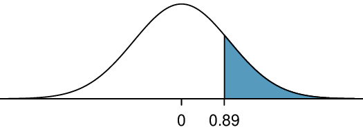
\begin{matrix} Z = \frac{point estimate - null value}{S E of estimate} = \frac{0.52 - 0.50}{0.022} = 0.89 \end{matrix}

🔗

Because the alternative hypothesis uses a greater than sign (

>

), this is an upper-tail test. We find the area under the standard normal curve to the right of

Z = 0.89 .

A figure featuring the p-value is shown in Figure 6.1.16 as the shaded region.

🔗

Figure 6.1.16. Sampling distribution of the sample proportion if the null hypothesis is true for Example 6.1.15. The p-value for the test is shaded.
🔗

Using a table or a calculator, we find the p-value is 0.19. This p-value of 0.19 is greater than

α = 0.05,

so we do not reject

H_{0} .

That is, we do not have sufficient evidence to support Toohey’s campaign manager’s claims that she has more than 50% support within the district.

🔗

Example 6.1.17.

Based on the result above, do we have evidence that Toohey’s support equals 50%?

🔗

Solution.

No. In a hypothesis test we look for degrees of evidence against the null hypothesis. We cannot ever prove the null hypothesis directly. The value 0.5 is reasonable, but many other values are reasonable as well. There are many values that would not get rejected by this test.

🔗

We now summarize the steps for carrying out a hypothesis test for a proportion using the five step framework introduced in the previous chapter.

🔗

Hypothesis testing for a proportion.

To carry out a complete hypothesis test to test the claim that a single proportion

p

is equal to a null value

p_{0},

🔗

Identify: Identify the hypotheses and the significance level,

α .

$H_{0} :$ $p = p_{0}$
🔗

🔗
$H_{A} :$ $p \neq p_{0};$ $H_{A} :$ $p > p_{0};$ or $H_{A} :$ $p < p_{0}$
🔗

🔗

🔗

Choose: Choose the correct test procedure and identify it by name.

Here we choose the 1-proportion Z-test.
🔗

🔗

🔗

Check: Check conditions for the sampling distribution of

\hat{p}

to be nearly normal.

Data come from a random sample.
🔗

🔗
$n p_{0} \geq 10$ and $n (1 - p_{0}) \geq 10$ (Make sure to plug in numbers.)
🔗

🔗

🔗

Calculate: Calculate the Z-statistic and p-value.

🔗

$Z = \frac{point estimate - null value}{S E of estimate}$
🔗
- point estimate: the sample proportion $\hat{p}$
  🔗
  
  🔗
- $S E$ of estimate: $\sqrt{\frac{p_{0} (1 - p_{0})}{n}}$
  🔗
  
  🔗
- null value: $p_{0}$
  🔗
  
  🔗
🔗
🔗
p-value = (based on the Z-statistic and the direction of $H_{A}$ )
🔗

🔗

🔗

Conclude: Compare the p-value to

α,

and draw a conclusion in context.

If the p-value is $< α,$ reject $H_{0};$ there is sufficient evidence that [ $H_{A}$ in context].
🔗

🔗
If the p-value is $> α,$ do not reject $H_{0};$ there is not sufficient evidence that [ $H_{A}$ in context].
🔗

🔗

🔗

Example 6.1.18.

A Gallup poll conducted in March of 2016 found that 54% of respondents oppose nuclear energy

⁹

https://news.gallup.com/poll/190064/first-time-majority-oppose-nuclear-energy.aspx

. This was the first time since Gallup first asked the question in 1994 that a majority of respondents said they oppose nuclear energy. The survey was based on telephone interviews from a random sample of 1,019 adults in the United States. Does this poll provide evidence that greater than half of U.S. adults oppose nuclear energy? Carry out an appropriate test at the 0.10 significance level. Use the five step framework to organize your work.

🔗

Solution.

Identify: We will test the following hypotheses at the

α = 10 %

significance level.

🔗

H_{0} :

p = 0.5

🔗

H_{A} :

p > 0.5

Greater than half of all U.S. adults oppose nuclear energy.

🔗

Note:

p > 0.5

is what we want to find evidence for; this bears the burden of proof, so this corresponds to

H_{A} .

🔗

Choose: Because the hypotheses are about a single proportion, we choose the 1-proportion Z-test.

🔗

Check: We must verify that the sample proportion can be modeled using a normal distribution. The problem states that the data come from a random sample. Also,

1019 (0.5) \geq 10

and

1019 (1 - 0.5) \geq 10

so both conditions are met. (Remember to use the hypothesized proportion, not the sample proportion, when checking the conditions for this test.)

🔗

Calculate: We will calculate the Z-statistic and the p-value.

\begin{matrix} Z = \frac{point estimate - null value}{S E of estimate} \end{matrix}

🔗

The point estimate is the sample proportion:

\hat{p} = 0.54 .

🔗

The value hypothesized for the parameter in

H_{0}

is the null value:

p_{0} = 0.5

🔗

The

S E

of the sample proportion, assuming

H_{0}

is true, is:

\sqrt{\frac{p_{0} (1 - p_{0})}{n}} = \sqrt{\frac{0.5 (1 - 0.5)}{1019}}

\begin{matrix} Z = \frac{0.54 - 0.5}{\sqrt{\frac{0.5 (1 - 0.5)}{1019}}} = 2.5 \end{matrix}

🔗

Because

H_{A}

uses a greater than sign (

>

), meaning that it is an upper-tail test, the p-value is the area to the right of

Z = 2.5

under the standard normal curve. This area can be found using a normal table or a calculator. The area or p-value =

0.006 .

🔗

Conclude: The p-value of 0.006 is

< 0.10,

so we reject

H_{0};

there is sufficient evidence that greater than half of U.S. adults oppose nuclear energy (as of March 2016).

🔗

Guided Practice 6.1.19.

In context, interpret the p-value of 0.006 from the previous example.

¹⁰

Assuming the normal model is accurate, there is a 0.006 probability of getting a test statistic greater than 2.5 if $H_{0}$ were true, that is, if the true proportion of U.S. adults that oppose nuclear energy really is 0.5. Note: We start by assuming

H_{0}

is true, that

p

really equals 0.5. Then, assuming this, we estimate the probability of getting a sample proportion of 0.54 or larger by finding the area under the standard normal curve to the right of 2.5. This probability is very small, which casts doubt on the null hypothesis and leads us to reject it.

🔗

Subsection 6.1.7 Calculator: the 1-proportion Z-test

A calculator can be useful for evaluating the test statistic and computing the p-value.

🔗

TI-83/84: 1-proportion Z-test.

Use STAT, TESTS, 1-PropZTest.

Choose STAT.
🔗

🔗
Right arrow to TESTS.
🔗

🔗
Down arrow and choose 5:1-PropZTest.
🔗

🔗
Let $p_{0}$ be the null or hypothesized value of p.
🔗

🔗
Let x be the number of yeses (must be an integer).
🔗

🔗
Let n be the sample size.
🔗

🔗
Choose $\neq,$ $<,$ or $>$ to correspond to $H_{A} .$
🔗

🔗
Choose Calculate and hit ENTER, which returns
🔗

z Z-statistic

p p-value

$\hat{p}$ the sample proportion

n the sample size

🔗

🔗

Casio fx-9750GII: 1-proportion Z-test.

The steps closely match those of the 1-proportion confidence interval.

Navigate to STAT (MENU button, then hit the 2 button or select STAT).
🔗

🔗
Choose the TEST option (F3 button).
🔗

🔗
Choose the Z option (F1 button).
🔗

🔗
Choose the 1-P option (F3 button).
🔗

🔗
Specify the test details:
- Specify the sidedness of the test using the F1, F2, and F3 keys.
  🔗
  
  🔗
- Enter the null value, p0.
  🔗
  
  🔗
- Enter the number of successes, x.
  🔗
  
  🔗
- Enter the sample size, n.
  🔗
  
  🔗
🔗
🔗
Hit the EXE button, which returns
🔗

z Z-statistic

p p-value

$\hat{p}$ the sample proportion

n the sample size

🔗

🔗

Guided Practice 6.1.20.

Using a calculator, find the test statistic and p-value for the earlier Example 6.1.18. Recall that we were looking for evidence that more than half of U.S. adults oppose nuclear energy. The sample percent was 54%, and the sample size was 1019.

¹¹

Navigate to the 1-proportion Z-test on the calculator. Let p0

= 0.5 .

To find x, do

0.54 \times 1019 = 550.26 .

This needs to be an integer, so round to the closest integer. Here x

= 550 .

Also, n

= 1019 .

We are looking for evidence that greater than half oppose, so choose > p0. When we do Calculate, we get the test statistic: Z = 2.64 and the p-value: p = 0.006.

🔗

Subsection 6.1.8 Section summary

Most of the confidence interval procedures and hypothesis tests of this book involve: a point estimate, the standard error of the point estimate, and an assumption about the shape of the sampling distribution of the point estimate. In this section, we explore inference when the parameter of interest is a proportion.

🔗

We use the sample proportion $\hat{p}$ as the point estimate for the unknown population proportion $p .$ The sampling distribution of $\hat{p}$ is approximately normal when the success-failure condition is met and the observations are independent. When the sampling distribution of $\hat{p}$ is normal, the standardized test statistic also follows a normal distribution.
🔗

🔗
When verifying the success-failure condition and calculating the $S E,$
🔗
- use the sample proportion $\hat{p}$ for the confidence interval, but
  🔗
  
  🔗
- use the null/hypothesized proportion $p_{0}$ for the hypothesis test.
  🔗
  
  🔗
🔗
🔗
When there is one sample and the parameter of interest is a single proportion:
- Estimate $p$ at the C% confidence level using a 1-proportion Z-interval.
  🔗
  
  🔗
- Test $H_{0} :$ $p = p_{0}$ at the $α$ significance level using a 1-proportion Z-test.
  🔗
  
  🔗
🔗
🔗
The one proportion Z-test and Z-interval require the sampling distribution for $\hat{p}$ to be nearly normal. For this reason we must check that the following conditions are met.
1. Independence: The data should come from a random sample or random process. When sampling without replacement, check that the sample size is less than 10% of the population size.
  🔗
  
  🔗
2. Success-failure for Interval: $n \hat{p} \geq 10$ and $n (1 - \hat{p}) \geq 10 .$
  🔗
  
  Success-failure for Test: assuming $H_{0} : p = p_{0}$ is true: $n p_{0} \geq 10$ and $n (1 - p_{0}) \geq 10 .$
  🔗
  
  🔗
🔗
🔗
When the conditions are met, we calculate the confidence interval and the test statistic as follows.
- Confidence interval: $point estimate \pm z^{⋆} \times S E of estimate$
  🔗
  
  🔗
- Test statistic: $Z = \frac{point estimate - null value}{S E of estimate}$
  🔗
  
  🔗
- Here the point estimate is the sample proportion $\hat{p} .$
  🔗
  
  🔗
- The $S E$ of estimate is the $S E$ of the sample proportion.
  - For an Interval, use $S E = \sqrt{\frac{\hat{p} (1 - \hat{p})}{n}}$
    🔗
    
    🔗
  - For a Test with $H_{0} : p = p_{0},$ use $S E = \sqrt{\frac{p_{0} (1 - p_{0})}{n}}$
    🔗
    
    🔗
  🔗
  🔗
🔗
🔗
The margin of error ( $M E$ ) for a one-sample confidence interval for a proportion is $z^{⋆} \sqrt{\frac{\hat{p} (1 - \hat{p})}{n}},$ which is proportional to $\frac{1}{\sqrt{n}} .$
🔗

🔗
To find the minimum sample size needed to estimate a proportion with a given confidence level and a given margin of error, $m,$ set up an inequality of the form:

$\begin{matrix} z^{⋆} \sqrt{\frac{\hat{p} (1 - \hat{p})}{n}} < m \end{matrix}$

$z^{⋆}$ depends on the desired confidence level. Unless a particular proportion is given in the problem, use $\hat{p} = 0.5 .$ We solve for the sample size $n .$ The final answer should be an integer, since $n$ refers to a number of people or things.

🔗

🔗

🔗

Exercises 6.1.9 Exercises

1. Orange tabbies.

Suppose that 90% of orange tabby cats are male. Determine if the following statements are true or false, and explain your reasoning.

The distribution of sample proportions of random samples of size 30 is left skewed.
🔗

🔗
Using a sample size that is 4 times as large will reduce the standard error of the sample proportion by one-half.
🔗

🔗
The distribution of sample proportions of random samples of size 140 is approximately normal.
🔗

🔗
The distribution of sample proportions of random samples of size 280 is approximately normal.
🔗

🔗

🔗

Solution.

True. See the reasoning of Exercise 4.1.5.3, part b.
🔗

🔗
True. We take the square root of the sample size in the SE formula.
🔗

🔗
True. The independence and success-failure conditions are satisfied.
🔗

🔗
True. The independence and success-failure conditions are satisfied.
🔗

🔗

🔗

2. Young Americans, Part II.

About 25% of young Americans have delayed starting a family due to the continued economic slump. Determine if the following statements are true or false, and explain your reasoning.

¹²

Demos.org. “The State of Young America: The Poll”. In: Demos (2011).

The distribution of sample proportions of young Americans who have delayed starting a family due to the continued economic slump in random samples of size 12 is right skewed.
🔗

🔗
In order for the distribution of sample proportions of young Americans who have delayed starting a family due to the continued economic slump to be approximately normal, we need random samples where the sample size is at least 40.
🔗

🔗
A random sample of 50 young Americans where 20% have delayed starting a family due to the continued economic slump would be considered unusual.
🔗

🔗
A random sample of 150 young Americans where 20% have delayed starting a family due to the continued economic slump would be considered unusual.
🔗

🔗
Tripling the sample size will reduce the standard error of the sample proportion by one-third.
🔗

🔗

🔗

3. Gender equality.

The General Social Survey asked a random sample of 1,390 Americans the following question: “On the whole, do you think it should or should not be the government’s responsibility to promote equality between men and women?” 82% of the respondents said it “should be”. At a 95% confidence level, this sample has 2% margin of error. Based on this information, determine if the following statements are true or false, and explain your reasoning.

¹³

National Opinion Research Center, General Social Survey, 2018.

We are 95% confident that between 80% and 84% of Americans in this sample think it’s the government’s responsibility to promote equality between men and women.
🔗

🔗
We are 95% confident that between 80% and 84% of all Americans think it’s the government’s responsibility to promote equality between men and women.
🔗

🔗
If we considered many random samples of 1,390 Americans, and we calculated 95% confidence intervals for each, 95% of these intervals would include the true population proportion of Americans who think it’s the government’s responsibility to promote equality between men and women.
🔗

🔗
In order to decrease the margin of error to 1%, we would need to quadruple (multiply by 4) the sample size.
🔗

🔗
Based on this confidence interval, there is sufficient evidence to conclude that a majority of Americans think it’s the government’s responsibility to promote equality between men and women.
🔗

🔗

🔗

Solution.

False. A confidence interval is constructed to estimate the population proportion, not the sample proportion.
🔗

🔗
True. 95% CI: $82 % \pm 2 % .$
🔗

🔗
True. By the definition of the confidence level.
🔗

🔗
True. Quadrupling the sample size decreases the SE and ME by a factor of $1 / \sqrt{4} .$
🔗

🔗
True. The 95% CI is entirely above 50%.
🔗

🔗

🔗

4. Elderly drivers.

The Marist Poll published a report stating that 66% of adults nationally think licensed drivers should be required to retake their road test once they reach 65 years of age. It was also reported that interviews were conducted on 1,018 American adults, and that the margin of error was 3% using a 95% confidence level.

¹⁴

Marist Poll, Road Rules: Re-Testing Drivers at Age 65?, March 4, 2011.

Verify the margin of error reported by The Marist Poll.
🔗

🔗
Based on a 95% confidence interval, does the poll provide convincing evidence that more than 70% of the population think that licensed drivers should be required to retake their road test once they turn 65?
🔗

🔗

🔗

5. Fireworks on July $4^{t h}$ .

A local news outlet reported that 56% of 600 randomly sampled Kansas residents planned to set off fireworks on July

4^{t h} .

Determine the margin of error for the 56% point estimate using a 95% confidence level.

¹⁵

Survey USA, News Poll #19333, data collected on June 27, 2012.

🔗

Solution.

With a random sample, independence is satisfied. The success-failure condition is also satisfied.

M E = z^{*} \sqrt{\frac{\hat{p} (1 - \hat{p})}{n}} = 1.96 \sqrt{\frac{0.56 \times 0.44}{600}} = 0.0397 \approx 4 %

🔗

6. Life rating in Greece.

Greece has faced a severe economic crisis since the end of 2009. A Gallup poll surveyed 1,000 randomly sampled Greeks in 2011 and found that 25% of them said they would rate their lives poorly enough to be considered “suffering”.

¹⁶

Gallup World, More Than One in 10 “Suffering” Worldwide, data collected throughout 2011.

Describe the population parameter of interest. What is the value of the point estimate of this parameter?
🔗

🔗
Check if the conditions required for constructing a confidence interval based on these data are met.
🔗

🔗
Construct a 95% confidence interval for the proportion of Greeks who are “suffering”.
🔗

🔗
Without doing any calculations, describe what would happen to the confidence interval if we decided to use a higher confidence level.
🔗

🔗
Without doing any calculations, describe what would happen to the confidence interval if we used a larger sample.
🔗

🔗

🔗

7. Study abroad.

A survey on 1,509 high school seniors who took the SAT and who completed an optional web survey shows that 55% of high school seniors are fairly certain that they will participate in a study abroad program in college.

¹⁷

studentPOLL, College-Bound Students’ Interests in Study Abroad and Other International Learning Activities, January 2008.

Is this sample a representative sample from the population of all high school seniors in the US? Explain your reasoning.
🔗

🔗
Let’s suppose the conditions for inference are met. Even if your answer to part (a) indicated that this approach would not be reliable, this analysis may still be interesting to carry out (though not report). Construct a 90% confidence interval for the proportion of high school seniors (of those who took the SAT) who are fairly certain they will participate in a study abroad program in college, and interpret this interval in context.
🔗

🔗
What does “90% confidence” mean?
🔗

🔗
Based on this interval, would it be appropriate to claim that the majority of high school seniors are fairly certain that they will participate in a study abroad program in college?
🔗

🔗

🔗

Solution.

No. The sample only represents student who took the SAT, and this was also an online survey.
🔗

🔗
$(0.5289, 0.5711) .$ We are 90% confident that 53% to 57% of high school seniors who took the SAT are fairly certain that they will participate in a study abroad program in college.
🔗

🔗
90% of such random samples would produce a 90% confidence interval that includes the true proportion.
🔗

🔗
Yes. The interval lies entirely above 50%.
🔗

🔗

🔗

8. Legalization of marijuana, Part I.

The General Social Survey asked 1,578 US residents: “Do you think the use of marijuana should be made legal, or not?” 61% of the respondents said it should be made legal.

¹⁸

National Opinion Research Center, General Social Survey, 2018

¹⁹

gss.norc.org/get-the-data

Is 61% a sample statistic or a population parameter? Explain.
🔗

🔗
Construct a 95% confidence interval for the proportion of US residents who think marijuana should be made legal, and interpret it in the context of the data.
🔗

🔗
A critic points out that this 95% confidence interval is only accurate if the statistic follows a normal distribution, or if the normal model is a good approximation. Is this true for these data? Explain.
🔗

🔗
A news piece on this survey’s findings states, “Majority of Americans think marijuana should be legalized.” Based on your confidence interval, is this news piece’s statement justified?
🔗

🔗

🔗

9. National Health Plan, Part I.

A Kaiser Family Foundation poll for US adults in 2019 found that 79% of Democrats, 55% of Independents, and 24% of Republicans supported a generic “National Health Plan”. There were 347 Democrats, 298 Republicans, and 617 Independents surveyed.

²⁰

Kaiser Family Foundation, The Public On Next Steps For The ACA And Proposals To Expand Coverage, data collected between Jan 9-14, 2019.

A political pundit on TV claims that a majority of Independents support a National Health Plan. Do these data provide strong evidence to support this type of statement?
🔗

🔗
Would you expect a confidence interval for the proportion of Independents who oppose the public option plan to include 0.5? Explain.
🔗

🔗

🔗

Solution.

We want to check for a majority (or minority), so we use the following hypotheses:

$\begin{aligned} H_{0} : p = 0.5 & H_{A} : p \neq 0.5 \end{aligned}$

We have a sample proportion of $\hat{p} = 0.55$ and a sample size of $n = 617$ independents.

🔗

Since this is a random sample, independence is satisfied. The success-failure condition is also satisfied: $617 \times 0.5$ and $617 \times (1 - 0.5)$ are both at least 10 (we use the null proportion $p_{0} = 0.5$ for this check in a one-proportion hypothesis test).
🔗

Therefore, we can model $\hat{p}$ using a normal distribution with a standard error of

$\begin{matrix} S E = \sqrt{\frac{p (1 - p)}{n}} = 0.02 \end{matrix}$

(We use the null proportion $p_{0} = 0.5$ to compute the standard error for a one-proportion hypothesis test.) Next, we compute the test statistic:

$\begin{matrix} Z = \frac{0.55 - 0.5}{0.02} = 2.5 \end{matrix}$

This yields a one-tail area of 0.0062, and a p-value of $2 \times 0.0062 = 0.0124 .$

🔗

Because the p-value is smaller than 0.05, we reject the null hypothesis. We have strong evidence that the support is different from 0.5, and since the data provide a point estimate above 0.5, we have strong evidence to support this claim by the TV pundit.
🔗

🔗
No. Generally we expect a hypothesis test and a confidence interval to align, so we would expect the confidence interval to show a range of plausible values entirely above 0.5. However, if the confidence level is misaligned (e.g. a 99% confidence level and a $α = 0.05$ significance level), then this is no longer generally true.
🔗

🔗

🔗

10. Is college worth it? Part I.

Among a simple random sample of 331 American adults who do not have a four-year college degree and are not currently enrolled in school, 48% said they decided not to go to college because they could not afford school.

²¹

Pew Research Center Publications, Is College Worth It?, data collected between March 15-29, 2011.

A newspaper article states that only a minority of the Americans who decide not to go to college do so because they cannot afford it and uses the point estimate from this survey as evidence. Conduct a hypothesis test to determine if these data provide strong evidence supporting this statement.
🔗

🔗
Would you expect a confidence interval for the proportion of American adults who decide not to go to college because they cannot afford it to include 0.5? Explain.
🔗

🔗

🔗

11. Taste test.

Some people claim that they can tell the difference between a diet soda and a regular soda in the first sip. A researcher wanting to test this claim randomly sampled 80 such people. He then filled 80 plain white cups with soda, half diet and half regular through random assignment, and asked each person to take one sip from their cup and identify the soda as diet or regular. 53 participants correctly identified the soda.

Do these data provide strong evidence that these people are any better or worse than random guessing at telling the difference between diet and regular soda?
🔗

🔗
Interpret the p-value in this context.
🔗

🔗

🔗

Solution.

Identify: $H_{0} : p = 0.5 .$ $H_{A} : p \neq 0.5 .$ Choose: 1-proportionZ-test. Check: Independence (random sample, $< 10 %$ of population) is satisfied, as is the success-failure conditions (using $p_{0} = 0.5,$ we expect 40 successes and 40 failures). $Z = 2.91 \to p-value = 0.0018 .$ Conlcude: Since the p-value $< 0.05,$ we reject the null hypothesis. The data provide strong evidence that the rate of correctly identifying a soda for these people is significantly better than just by random guessing.
🔗

🔗
The p-value represents the following conditional probability: $P (\hat{p} > 0.6625 | p = 0.5) .$ If in fact people cannot tell the difference between diet and regular soda and they randomly guess, the probability of getting a random sample of 80 people where 66.25% (53/80) or higher identify a soda correctly would be 0.0018.
🔗

🔗

🔗

12. Is college worth it? Part II.

Exercise 6.1.9.10 presents the results of a poll where 48% of 331 Americans who decide to not go to college do so because they cannot afford it.

Calculate a 90% confidence interval for the proportion of Americans who decide to not go to college because they cannot afford it, and interpret the interval in context.
🔗

🔗
Suppose we wanted the margin of error for the 90% confidence level to be about 1.5%. How large of a survey would you recommend?
🔗

🔗

🔗

13. National Health Plan, Part II.

Exercise 6.1.9.9 presents the results of a poll evaluating support for a generic “National Health Plan” in the US in 2019, reporting that 55% of Independents are supportive. If we wanted to estimate this number to within 1% with 90% confidence, what would be an appropriate sample size?

🔗

Solution.

Since a sample proportion (

\hat{p} = 0.55

) is available, we use this for the sample size calculations. The margin of error for a 90% confidence interval is

1.6449 \times S E = 1.6449 \times \sqrt{\frac{p (1 - p)}{n}} .

We want this to be less than 0.01, where we use

\hat{p}

in place of

p :

\begin{matrix} 1.6449 \times \sqrt{\frac{0.55 (1 - 0.55)}{n}} < 0.01 \\ {1.6449}^{2} \frac{0.55 (1 - 0.55)}{{0.01}^{2}} < n \end{matrix}

From this, we get that

n

must be at least 6697.

🔗

14. Legalize Marijuana, Part II.

As discussed in Exercise 6.1.9.8, the General Social Survey reported a sample where about 61% of US residents thought marijuana should be made legal. If we wanted to limit the margin of error of a 95% confidence interval to 2%, about how many Americans would we need to survey?

🔗

You have attempted 1 of 2 activities on this page.

🔗

Prev Top Next

(,)	the confidence interval
$\hat{p}$	the sample proportion
`n`	the sample size

`Left`, `Right`	ends of the confidence interval
$\hat{p}$	sample proportion
`n`	sample size

`z`	Z-statistic
`p`	p-value
$\hat{p}$	the sample proportion
`n`	the sample size

Section 6.1 Inference for a single proportion

Objectives: Learning objectives

Subsection 6.1.1 Distribution of a sample proportion (review)

Conditions for the sampling distribution of p^ being nearly normal.

Subsection 6.1.2 Checking conditions for inference using a normal distribution

Subsection 6.1.3 Confidence intervals for a proportion

Example 6.1.1.

Example 6.1.2.

Example 6.1.3.

Example 6.1.4.

Example 6.1.5.

Example 6.1.6.

Constructing a confidence interval for a proportion.

Example 6.1.7.

Guided Practice 6.1.8.

Subsection 6.1.4 Calculator: the 1-proportion Z-interval

TI-83/84: 1-proportion Z-interval.

Casio fx-9750GII: 1-proportion Z-interval.

Guided Practice 6.1.9.

Subsection 6.1.5 Choosing a sample size when estimating a proportion

Margin of error.

Example 6.1.10.

Example 6.1.11.

Identify a sample size for a particular margin of error.

Guided Practice 6.1.12.

Guided Practice 6.1.13.

Subsection 6.1.6 Hypothesis testing for a proportion

Example 6.1.14.

Confidence intervals versus hypothesis tests for a single proportion.

Example 6.1.15.

Example 6.1.17.

Hypothesis testing for a proportion.

Example 6.1.18.

Guided Practice 6.1.19.

Subsection 6.1.7 Calculator: the 1-proportion Z-test

TI-83/84: 1-proportion Z-test.

Casio fx-9750GII: 1-proportion Z-test.

Guided Practice 6.1.20.

Subsection 6.1.8 Section summary

Exercises 6.1.9 Exercises

1. Orange tabbies.

2. Young Americans, Part II.

3. Gender equality.

4. Elderly drivers.

5. Fireworks on July 4th.

6. Life rating in Greece.

7. Study abroad.

8. Legalization of marijuana, Part I.

9. National Health Plan, Part I.

10. Is college worth it? Part I.

11. Taste test.

12. Is college worth it? Part II.

13. National Health Plan, Part II.

14. Legalize Marijuana, Part II.

Conditions for the sampling distribution of $\hat{p}$ being nearly normal.

5. Fireworks on July $4^{t h}$ .