Objectives: Learning objectives
-
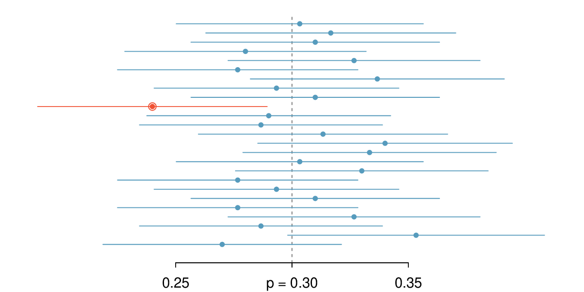
Explain the purpose and use of confidence intervals.
-
Construct 95% confidence intervals assuming the point estimate follows a normal distribution.
-
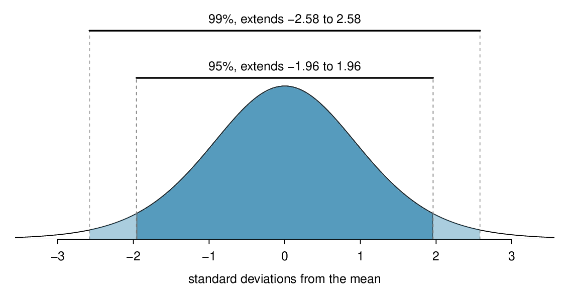
Calculate the critical value for a C% confidence interval when the point estimate follows a normal distribution.
-
Describe how sample size and confidence level affect the width of a confidence interval.
-
Interpret a confidence interval and the confidence level in context.
-
Draw conclusions with a specified confidence level about the values of unknown parameters.
-
Calculate and interpret the margin of error for a C% confidence interval. Distinguish between margin of error and standard error.