
Advanced High School Statistics: Third Edition

Section 6.3 Testing for goodness of fit using chi-square

In this section, we develop a method for assessing a null model when the data take on more than two categories, such as yes/no/maybe instead of simply yes/no. This allows us to answer questions such as the following:
  • Are juries representative of the population in terms of race/ethnicity, or is there a bias in jury selection?
  • Is the color distribution of actual M&M’s consistent with what was reported on the Mars website?
  • Do people choose rock, paper, scissors with the same likelihood, or is one choice favored over another?

Subsection 6.3.1 Creating a test statistic for one-way tables

Data is collected from a random sample of 275 jurors in a small county. Jurors identified their racial group, as shown in Table 6.3.1, and we would like to determine if these jurors are racially representative of the population. If the jury is representative of the population, then the proportions in the sample should roughly reflect the population of eligible jurors, i.e. registered voters.
Table 6.3.1. Representation by race in a city’s juries and population.
Race/Ethnicity White Black Hispanic Other Total
Representation in juries 205 26 25 19 275
Registered voters 0.72 0.07 0.12 0.09 1.00
While the proportions in the juries do not precisely represent the population proportions, it is unclear whether these data provide convincing evidence that the sample is not representative. If the jurors really were randomly sampled from the registered voters, we might expect small differences due to chance. However, unusually large differences may provide convincing evidence that the juries were not representative.

Example 6.3.2.

Of the people in the city, 275 served on a jury. If the individuals are randomly selected to serve on a jury, about how many of the 275 people would we expect to be white? How many would we expect to be black?
Solution.
About 72% of the population is white, so we would expect about 72% of the jurors to be white: \(0.72\times 275 = 198\text{.}\)
Similarly, we would expect about 7% of the jurors to be black, which would correspond to about \(0.07\times 275 = 19.25\) black jurors.

Guided Practice 6.3.3.

Twelve percent of the population is Hispanic and 9% represent other races. How many of the 275 jurors would we expect to be Hispanic or from another race? Answers can be found in Table 6.3.4.
Table 6.3.4. Actual and expected make-up of the jurors.
Race/Ethnicity White Black Hispanic Other Total
Observed data 205 26 25 19 275
Expected counts 198 19.25 33 24.75 275
The sample proportion represented from each race among the 275 jurors was not a precise match for any ethnic group. While some sampling variation is expected, we would expect the sample proportions to be fairly similar to the population proportions if there is no bias on juries. We need to test whether the differences are strong enough to provide convincing evidence that the jurors are not a random sample. These ideas can be organized into hypotheses:
  • \(H_{0}\text{:}\) The jurors are a random sample, i.e. there is no racial/ethnic bias in who serves on a jury, and the observed counts reflect natural sampling fluctuation.
  • \(H_{A}\text{:}\) The jurors are not randomly sampled, i.e. there is racial/ethnic bias in juror selection.
To evaluate these hypotheses, we quantify how different the observed counts are from the expected counts. Strong evidence for the alternative hypothesis would come in the form of unusually large deviations in the groups from what would be expected based on sampling variation alone.

Subsection 6.3.2 The chi-square test statistic

In previous hypothesis tests, we constructed a test statistic of the following form:
\begin{equation*} Z = \frac{\text{ point estimate } - \text{ null value } }{SE \text{ of point estimate } } \end{equation*}
This construction was based on (1) identifying the difference between a point estimate and an expected value if the null hypothesis was true, and (2) standardizing that difference using the standard error of the point estimate. These two ideas will help in the construction of an appropriate test statistic for count data.
In this example we have four categories: White, Black, Hispanic, and other. Because we have four values rather than just one or two, we need a new tool to analyze the data. Our strategy will be to find a test statistic that measures the overall deviation between the observed and the expected counts. We first find the difference between the observed and expected counts for the four groups:
\begin{align*} \amp \amp \text{ White } \amp \amp \text{ Black } \amp \amp \text{ Hispanic } \amp \amp \text{ Other }\\ \text{ observed - expected } \amp \amp 205-198 \amp \amp 26-19.25 \amp \amp 25-33 \amp \amp 19-24.75 \end{align*}
Next, we square the differences:
\begin{align*} \amp \amp \text{ White } \amp \amp \text{ Black } \amp \amp \text{ Hispanic } \amp \amp \text{ Other }\\ \text{ (observed - expected) } ^2 \amp \amp (205-198)^2 \amp \amp (26-19.25)^2 \amp \amp (25-33)^2 \amp \amp (19-24.75)^2 \end{align*}
We must standardize each term. To know whether the squared difference is large, we compare it to what was expected. If the expected count was 5, a squared difference of 25 is very large. However, if the expected count was 1,000, a squared difference of 25 is very small. We will divide each of the squared differences by the corresponding expected count.
\begin{align*} \amp \amp \text{ White } \amp \amp \text{ Black } \amp \amp \text{ Hispanic } \amp \amp \text{ Other }\\ \frac{\text{ (observed - expected) } ^2}{\text{ expected } } \amp \amp \frac{(205-198)^2}{198} \amp \amp \frac{(26-19.25)^2 }{19.25} \amp \amp \frac{(25-33)^2}{33} \amp \amp \frac{(19-24.75)^2}{24.75} \end{align*}
Finally, to arrive at the overall measure of deviation between the observed counts and the expected counts, we add up the terms.
\begin{align*} \chi^2 \amp = \sum{\frac{\text{ (observed - expected) } ^2}{\text{ expected } }}\\ \amp = \frac{(205-198)^2}{198} + \frac{(26-19.25)^2 }{19.25} + \frac{(25-33)^2}{33} + \frac{(19-24.75)^2}{24.75} \end{align*}
We can write an equation for \(\chi^2\) using the observed counts and expected counts:
\begin{align*} \chi^2 \amp = \frac {\text{\((\text{ observed count }_1 - \text{ expected count }_1)^2\)} } {\text{\(\text{ expected count }_1\)} } + \dots + \frac {\text{\((\text{ observed count }_4 - \text{ expected count }_4)^2\)} } {\text{\(\text{ expected count }_4\)} } \end{align*}
The final number \(\chi^2\) summarizes how strongly the observed counts tend to deviate from the null counts.
In Subsection 6.3.4, we will see that if the null hypothesis is true, then \(\chi^2\) follows a new distribution called a chi-square distribution. Using this distribution, we will be able to obtain a p-value to evaluate whether there appears to be racial/ethnic bias in the juries for the city we are considering.

Subsection 6.3.3 The chi-square distribution and finding areas

The chi-square distribution is sometimes used to characterize data sets and statistics that are always positive and typically right skewed. Recall a normal distribution had two parameters — mean and standard deviation — that could be used to describe its exact characteristics. The chi-square distribution has just one parameter called degrees of freedom (df), which influences the shape, center, and spread of the distribution.

Guided Practice 6.3.5.

Figure 6.3.6 shows three chi-square distributions. (a) How does the center of the distribution change when the degrees of freedom is larger? (b) What about the variability (spread)? (c) How does the shape change?
 1 
(a) The center becomes larger. If we look carefully, we can see that the center of each distribution is equal to the distribution’s degrees of freedom. (b) The variability increases as the degrees of freedom increases. (c) The distribution is very strongly right skewed for \(df=2\text{,}\) and then the distributions become more symmetric for the larger degrees of freedom \(df=4\) and \(df=9\text{.}\) In fact, as the degrees of freedom increase, the \(\chi^2\) distribution approaches a normal distribution.
Figure 6.3.6. Three chi-square distributions with varying degrees of freedom.
Figure 6.3.6 and Guided Practice 6.3.5 demonstrate three general properties of chi-square distributions as the degrees of freedom increases: the distribution becomes more symmetric, the center moves to the right, and the variability inflates.
Our principal interest in the chi-square distribution is the calculation of p-values, which (as we have seen before) is related to finding the relevant area in the tail of a distribution. To do so, a new table is needed: the chi-square table, partially shown in Table 6.3.7. A more complete table is presented in Table B.4.8. This table is very similar to the \(t\)-table from Section 7.1 and Section 7.3: we identify a range for the area, and we examine a particular row for distributions with different degrees of freedom. One important difference from the \(t\)-table is that the chi-square table only provides upper tail values.
Table 6.3.7. A section of the chi-square table. A complete table is in Table B.4.8.
Upper tail 0.3 0.2 0.1 0.05 0.02 0.01 0.005 0.001
df 1 1.07 1.64 2.71 3.84 5.41 6.63 7.88 10.83
2 2.41 3.22 4.61 5.99 7.82 9.21 10.60 13.82
3 3.66 4.64 6.25 7.81 9.84 11.34 12.84 16.27
4 4.88 5.99 7.78 9.49 11.67 13.28 14.86 18.47
5 6.06 7.29 9.24 11.07 13.39 15.09 16.75 20.52
6 7.23 8.56 10.64 12.59 15.03 16.81 18.55 22.46
7 8.38 9.80 12.02 14.07 16.62 18.48 20.28 24.32

Example 6.3.8.

Figure 6.3.(a) shows a chi-square distribution with 3 degrees of freedom and an upper shaded tail starting at 6.25. Use Table 6.3.7 to estimate the shaded area.
Solution.
This distribution has three degrees of freedom, so only the row with 3 degrees of freedom (df) is relevant. This row has been italicized in the table. Next, we see that the value — 6.25 — falls in the column with upper tail area 0.1. That is, the shaded upper tail of Figure 6.3.(a) has area 0.1.
(a)
(b)
(c)
(d)
(e)
(f)
Figure 6.3.9. Figure 6.3.(a) is a Chi-square distribution with 3 degrees of freedom, area above 6.25 shaded. Figure 6.3.(b) is 2 degrees of freedom, area above 4.3 shaded. Figure 6.3.(c) is 5 degrees of freedom, area above 5.1 shaded. Figure 6.3.(d) is 7 degrees of freedom, area above 11.7 shaded. Figure 6.3.(e) is 4 degrees of freedom, area above 10 shaded. Figure 6.3.(f) is 3 degrees of freedom, area above 9.21 shaded.

Example 6.3.10.

We rarely observe the exact value in the table. For instance, Figure 6.3.(b) shows the upper tail of a chi-square distribution with 2 degrees of freedom. The lower bound for this upper tail is at 4.3, which does not fall in Table 6.3.7. Find the approximate tail area.
Solution.
The cutoff 4.3 falls between the second and third columns in the 2 degrees of freedom row. Because these columns correspond to tail areas of 0.2 and 0.1, we can be certain that the area shaded in Figure 6.3.(b) is between 0.1 and 0.2.
Using a calculator or statistical software allows us to get more precise areas under the chi-square curve than we can get from the table alone.

TI-84: Finding an upper tail area under the chi-square curve.

Use the \(\chi^2\)cdf command to find areas under the chi-square curve.
  1. Hit 2ND VARS (i.e. DISTR).
  2. Choose 8:\(\chi^2\)cdf.
  3. Enter the lower bound, which is generally the chi-square value.
  4. Enter the upper bound. Use a large number, such as 1000.
  5. Enter the degrees of freedom.
  6. Choose Paste and hit ENTER.
TI-83: Do steps 1-2, then type the lower bound, upper bound, and degrees of freedom separated by commas. e.g. \(\chi^2\)cdf(5, 1000, 3), and hit ENTER.

Casio fx-9750GII: Finding an upper tail area under the chi-sq. curve.

  1. Navigate to STAT (MENU button, then hit the 2 button or select STAT).
  2. Choose the DIST option (F5 button).
  3. Choose the CHI option (F3 button).
  4. Choose the Ccd option (F2 button).
  5. If necessary, select the Var option (F2 button).
  6. Enter the Lower bound (generally the chi-square value).
  7. Enter the Upper bound (use a large number, such as 1000).
  8. Enter the degrees of freedom, df.
  9. Hit the EXE button.

Guided Practice 6.3.11.

Figure 6.3.(c) shows an upper tail for a chi-square distribution with 5 degrees of freedom and a cutoff of 5.1. Find the tail area using a calculator.
 2 
Use a lower bound of \(5.1\text{,}\) an upper bound of 1000, and \(df = 5\text{.}\) The upper tail area is 0.4038.

Guided Practice 6.3.12.

Figure 6.3.(d) shows a cutoff of 11.7 on a chi-square distribution with 7 degrees of freedom. Find the area of the upper tail.
 3 
The area is 0.1109.

Guided Practice 6.3.13.

Figure 6.3.(e) shows a cutoff of 10 on a chi-square distribution with 4 degrees of freedom. Find the area of the upper tail.
 4 
The area is 0.4043.

Guided Practice 6.3.14.

Figure 6.3.(f) shows a cutoff of 9.21 with a chi-square distribution with 3 df. Find the area of the upper tail.
 5 
The area is 0.0266.

Subsection 6.3.4 Finding a p-value for a chi-square distribution

In Subsection 6.3.2, we identified a new test statistic (\(\chi^2\)) within the context of assessing whether there was evidence of racial/ethnic bias in how jurors were sampled. The null hypothesis represented the claim that jurors were randomly sampled and there was no racial/ethnic bias. The alternative hypothesis was that there was racial/ethnic bias in how the jurors were sampled.
We determined that a large \(\chi^2\) value would suggest strong evidence favoring the alternative hypothesis: that there was racial/ethnic bias. However, we could not quantify what the chance was of observing such a large test statistic (\(\chi^2=5.89\)) if the null hypothesis actually was true. This is where the chi-square distribution becomes useful. If the null hypothesis was true and there was no racial/ethnic bias, then \(\chi^2\) would follow a chi-square distribution, with three degrees of freedom in this case. Under certain conditions, the statistic \(\chi^2\) follows a chi-square distribution with \(k-1\) degrees of freedom, where \(k\) is the number of bins or categories of the variable.

Example 6.3.15.

How many categories were there in the juror example? How many degrees of freedom should be associated with the chi-square distribution used for \(\chi^2\text{?}\)
Solution.
In the jurors example, there were \(k=4\) categories: White, Black, Hispanic, and other. According to the rule above, the test statistic \(\chi^2\) should then follow a chi-square distribution with \(k-1 = 3\) degrees of freedom if \(H_0\) is true.
Just like we checked sample size conditions to use the normal model in earlier sections, we must also check a sample size condition to safely model \(\chi^2\) with a chi-square distribution. Each expected count must be at least 5. In the juror example, the expected counts were 198, 19.25, 33, and 24.75, all easily above 5, so we can model the \(\chi^2\) test statistic, using a chi-square distribution.

Example 6.3.16.

If the null hypothesis is true, the test statistic \(\chi^2=5.89\) would be closely associated with a chi-square distribution with three degrees of freedom. Using this distribution and test statistic, identify the p-value and state whether or not there is evidence of racial/ethnic bias in the juror selection.
Solution.
The chi-square distribution and p-value are shown in Figure 6.3.17. Because larger chi-square values correspond to stronger evidence against the null hypothesis, we shade the upper tail to represent the p-value. Using a calculator, we look at the chi-square curve with 3 degrees of freedom and find the area to the right of \(\chi^2=5.89\text{.}\) This area, which corresponds to the p-value, is equal to 0.117. This p-value is larger than the default significance level of 0.05, so we reject the null hypothesis. In other words, the data do not provide convincing evidence of racial/ethnic bias in the juror selection.
Figure 6.3.17. The p-value for the juror hypothesis test is shaded in the chi-square distribution with \(df=3\text{.}\)
The test that we just carried out regarding jury selection is known as the \(\chi^2\) goodness of fit test. It is called “goodness of fit” because we test whether or not the proposed or expected distribution is a good fit for the observed data.

Chi-square goodness of fit test for one-way table.

Suppose we are to evaluate whether there is convincing evidence that a set of observed counts \(O_1\text{,}\) \(O_2\text{,}\) ..., \(O_k\) in \(k\) categories are unusually different from what might be expected under a null hypothesis. Calculate the expected counts that are based on the null hypothesis \(E_1\text{,}\) \(E_2\text{,}\) ..., \(E_k\text{.}\) If each expected count is at least 5 and the null hypothesis is true, then the test statistic below follows a chi-square distribution with \(k-1\) degrees of freedom:
\begin{gather*} \chi^2 = \frac{(O_1 - E_1)^2}{E_1} + \frac{(O_2 - E_2)^2}{E_2} + \cdots + \frac{(O_k - E_k)^2}{E_k} \end{gather*}
The p-value for this test statistic is found by looking at the upper tail of this chi-square distribution. We consider the upper tail because larger values of \(\chi^2\) would provide greater evidence against the null hypothesis.

Conditions for the chi-square goodness of fit test.

The chi-square goodness of fit test requires two assumptions. The assumptions and the conditions that we check are listed below. If the conditions are not met, this test should not be used.
Independent. The observations can be considered independent if the data come from a random process. If randomly sampling from a finite population, the observations can be considered independent if sampling less than 10% of the population.
Sampling distribution is chi-square. In order for the \(\chi^2\)-statistic to follow the chi-square distribution, each particular bin or category must have at least 5 expected cases under the assumption that the null hypothesis is true.

Subsection 6.3.5 Evaluating goodness of fit for a distribution

Goodness of fit test for a one-way table.

When there is one sample and we are comparing the distribution of a categorical variable to a specified or population distribution, e.g. using sample values to determine if a machine is producing M&M’s with the specified distribution of color,
Identify: Identify the hypotheses and the significance level, \(\alpha\text{.}\)
  • \(H_0\text{:}\) The distribution of [...] matches the specified or population distribution.
  • \(H_A\text{:}\) The distribution of [...] doesn’t match the specified or population distribution.
Choose: Choose the correct test procedure and identify it by name.
  • Here we choose the \(\chi^2\) goodness of fit test.
Check: Check that the test statistic follows a chi-square distribution.
  1. Independence: Data come from a random sample or random process. If sampling without replacement, check that the sample size is less than 10% of the population size.
  2. All expected counts are \(\ge\) 5.
Calculate: Calculate the \(\chi^2\)-statistic, \(df\text{,}\) and p-value.
  • test statistic: \(\chi^2 =\sum{ \frac{\text{ (observed } - \text{ expected } )^2}{\text{ expected } }}\)
  • \(df =\) # of categories \(-1\)
  • p-value = (area to the right of \(\chi^2\)-statistic with the appropriate \(df\))
Conclude: Compare the p-value to \(\alpha\text{,}\) and draw a conclusion in context.
  • If the p-value is \(\lt \alpha\text{,}\) reject \(H_0\text{;}\) there is sufficient evidence that [\(H_A\) in context].
  • If the p-value is \(> \alpha\text{,}\) do not reject \(H_0\text{;}\) there is not sufficient evidence that [\(H_A\) in context].
Have you ever wondered about the color distribution of M&M’s©? If so, then you will be glad to know that Rick Wicklin, a statistician working at the statistical software company SAS, wondered about this too. But he did more than wonder; he decided to collect data to test whether the distribution of M&M colors was consistent with the stated distribution published on the Mars website in 2008. Starting at end of 2016, over the course of several weeks, he collected a sample of 712 candies, or about 1.5 pounds. We will investigate his results in the next example. You can read about his adventure in the Quartz article cited in the footnote below.
 6 

Example 6.3.18.

The stated color distribution of M&M’s on the Mars website in 2008 is shown in the table below, along with the observed percentages from Rick Wicklin’s sample of size 712. (See the paragraph before this example for more background.)
Blue Orange Green Yellow Red Brown
website percentages (2008): 24% 20% 16% 14% 13% 13%
observed percentages: 18.7% 18.7% 19.5% 14.5% 15.1% 13.5%
Is there evidence at the 5% significance level that the distribution of M&M’s in 2016 were different from the stated distribution on the website in 2008? Use the five step framework to organize your work.
Solution.
Identify: We will test the following hypotheses at the \(\alpha=0.05\) significance level.
\(H_0\text{:}\) The distribution of M&M colors is the same as the stated distribution in 2008.
\(H_A\text{:}\) The distribution of M&M colors is different than the stated distribution in 2008.
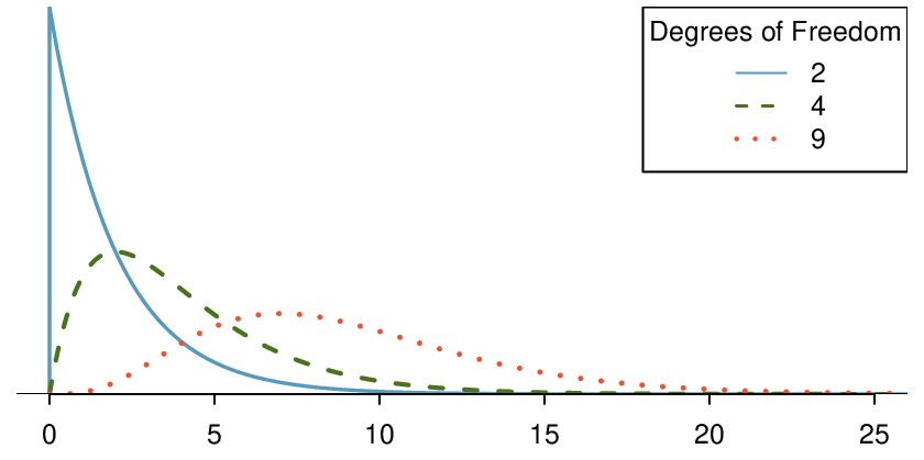
Choose: Because we have one variable (color), broken up into multiple categories, we choose the chi-square goodness of fit test.
Check: We must verify that the test statistic follows a chi-square distribution. Note that there is only one sample here. The website percentages are considered fixed — they are not the result of a sample and do not have sampling variability associated with them. To carry out the chi-square goodness of fit test, we will have to assume that Wicklin’s sample can be considered a random sample of M&M’s. We note that the total population size of M&M’s is much larger than 10 times the sample size of 712. Next, we need to find the expected counts. Here, \(n=712\text{.}\) If \(H_0\) is true, then we would expect 24% of the M&M’s to be Blue, 20% to be Orange, etc. So the expected counts can be found as:
Blue Orange Green Yellow Red Brown
expected counts: 0.24(712) 0.20(712) 0.16(712) 0.14(712) 0.13(712) 0.13(712)
= 170.9 = 142.4 = 113.9 = 99.6 = 92.6 = 92.6
Calculate: We will calculate the chi-square statistic, degrees of freedom, and the p-value.
To calculate the chi-square statistic, we need the observed counts as well as the expected counts. To find the observed counts, we use the observed percentages. For example, 18.7% of \(712 = 0.187(712)=133\text{.}\)
Blue Orange Green Yellow Red Brown
observed counts: 133 133 139 103 108 96
expected counts: 170.9 142.4 113.9 99.6 92.6 92.6
\begin{align*} \chi^2 =\amp \sum{\frac{\text{ (observed } - \text{ expected } )^2} {\text{ expected } }}\\ =\amp \frac{(133 - 170.9)^2}{170.9} + \frac{(133 - 142.4)^2}{142.4} + \cdots + \frac{(108 - 92.6)^2}{92.6} + \frac{(96 - 92.6)^2}{92.6}\\ =\amp 8.41+0.62+5.53+0.12+2.56+0.12\\ =\amp 17.36 \end{align*}
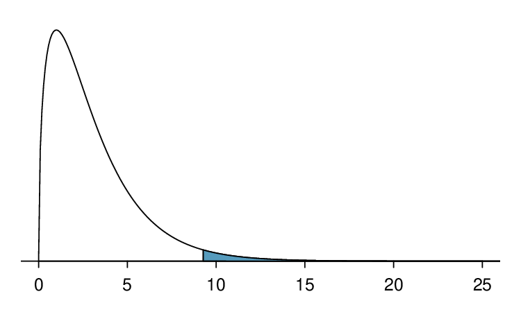
Because there are six colors, the degrees of freedom is 
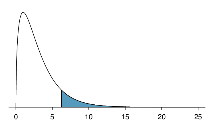
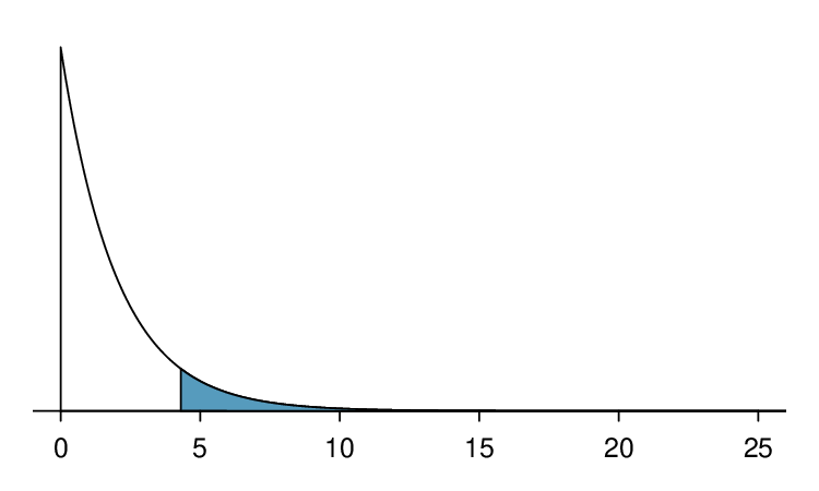
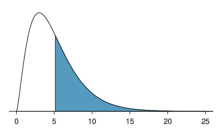
\(6-1=5\text{.}\) In a chi-square test, the p-value is always the area to the right of the chi-square statistic. Here, the area to the right of 17.36 under the chi-square curve with 5 degrees of freedom is \(0.004\text{.}\)
Conclude: The p-value of 0.004 is \(\lt 0.05\text{,}\) so we reject \(H_0\text{;}\) there is sufficient evidence that the distribution of M&M’s does not match the stated distribution on the website in 2008.

Example 6.3.19.

For Wicklin’s sample, which color showed the most prominent difference from the stated website distribution in 2008?
Solution.
We can compare the website percentages with the observed percentages. However, another approach is to look at the terms used when calculating the chi-square statistic. We note that the largest term, 8.41, corresponds to Blue. This means that the observed number for Blue was, relatively speaking, the farthest from the expected number among all of the colors. This is consistent with the observation that the largest difference in website percentage and observed percentage is for Blue (24% vs 18.7%). Wicklin observed far fewer Blue M&M’s than would have been expected if the website percentages were still true.

Subsection 6.3.6 Calculator: chi-square goodness of fit test

TI-84: Chi-square goodness of fit test.

Use STAT, TESTS, \(\chi^2\)GOF-Test.
  1. Enter the observed counts into list L1 and the expected counts into list L2.
  2. Choose STAT.
  3. Right arrow to TESTS.
  4. Down arrow and choose D:\(\chi^2\)GOF-Test.
  5. Leave Observed: L1 and Expected: L2.
  6. Enter the degrees of freedom after df:
  7. Choose Calculate and hit ENTER, which returns:
    \(\chi^2\) chi-square test statistic
    p p-value
    df degrees of freedom
TI-83: Unfortunately the TI-83 does not have this test built in. To carry out the test manually, make list L3 = (L1 - L2)\(^2\) / L2 and do 1-Var-Stats on L3. The sum of L3 will correspond to the value of \(\chi^2\) for this test.

Casio fx-9750GII: Chi-square goodness of fit test.

  1. Navigate to STAT (MENU button, then hit the 2 button or select STAT).
  2. Enter the observed counts into a list (e.g. List 1) and the expected counts into list (e.g. List 2).
  3. Choose the TEST option (F3 button).
  4. Choose the CHI option (F3 button).
  5. Choose the GOF option (F1 button).
  6. Adjust the Observed and Expected lists to the corresponding list numbers from Step 2.
  7. Enter the degrees of freedom, df.
  8. Specify a list where the contributions to the test statistic will be reported using CNTRB. This list number should be different from the others.
  9. Hit the EXE button, which returns
    \(\chi^2\) chi-square test statistic
    p p-value
    df degrees of freedom
    CNTRB list showing the test statistic contributions

Guided Practice 6.3.20.

Use the table below and a calculator to find the \(\chi^2\)-statistic and p-value for chi-square goodness of fit test.
 7 
Enter the observed counts into L1 and the expected counts into L2. the GOF test. Make sure that Observed: is L1 and Expected: is L2. Let df: be 5. You should find that \(\chi^{2} = 17.36\) and p-value \(= 0.004\text{.}\)
Blue Orange Green Yellow Red Brown
observed counts: 133 133 139 103 108 96
expected counts: 170.9 142.4 113.9 99.6 92.6 92.6

Subsection 6.3.7 Section summary

The inferential procedures we saw in the first two sections of this chapter are based on the test statistic following a normal distribution. In this section, we introduce a new distribution called the chi-square distribution.
  • While a normal distribution is defined by its mean and standard deviation, the chi-square distribution is defined by just one parameter called degrees of freedom.
  • For a chi-square distribution, as the degrees of freedom increases the center increases, the spread increases, and the shape becomes more symmetric and more normal.
     8 
    Technically, however, it is always right skewed.
  • When we want to see if a model is a good fit for observed data or if data is representative of a particular population, we can use a \(\chi^2\) goodness of fit test. This test is used when there is one variable with multiple categories (bins) that can be arranged in a one-way table.
  • In a chi-square goodness of fit test, we calculate a \(\chi^2\)-statistic, which is a measure of how far the observed values in the sample are from the expected values under the null hypothesis. \(\chi^2 =\sum{ \frac{\text{ (observed } - \text{ expected } )^2}{\text{ expected } }}\)
    • Always use whole numbers (counts) for the observed values, not proportions or percents.
    • For each category, the expected counts can be found by multiplying the sample size by the expected proportion under the null hypothesis. Expected counts do not need to be integers.
  • A larger \(\chi^2\) represents greater deviation between the observed values and the expected values under the null hypothesis. For a fixed degrees of freedom, a larger \(\chi^2\) value leads to a smaller p-value, providing greater evidence against \(H_0\text{.}\)
  • \(\chi^2\) tests for a one-way table. When there is one sample and we are comparing the distribution of a categorical variable to a specified or population distribution, e.g. using sample values to determine if a machine is producing M&M’s with the specified distribution of color, the hypotheses can often be written as:
    • \(H_0\text{:}\) The distribution of [...] matches the specified or population distribution.
    • \(H_A\text{:}\) The distribution of [...] doesn’t match the specified or population distribution.
    We test these hypotheses at the \(\alpha\) significance level using a \(\chi^2\) goodness of fit test.
  • For the \(\chi^2\) goodness of fit test, we check the following conditions to verify that the test statistic follows a chi-square distribution.
    1. Independence: Data come from a random sample or random process. When sampling without replacement, check that sample size is less than 10% of the population size.
    2. Expected counts: All expected counts are \(\ge\) 5.
  • We calculate the test statistic as follows:
    • test statistic: \(\chi^2 =\sum{ \frac{\text{ (observed} - \text{expected} )^2}{\text{ expected } }}\text{;}\) \(df =\) # of categories \(-1\)
  • The p-value is the area to the right of the \(\chi^2\)-statistic under the chi-square curve with the appropriate \(df\text{.}\)
  • For a \(\chi^2\) test, the p-value corresponds to the probability of getting a test statistic as large as we got or larger, assuming the null hypothesis is true and assuming the chi-square model holds.

Exercises 6.3.8 Exercises

1. True or false, Part I.

Determine if the statements below are true or false. For each false statement, suggest an alternative wording to make it a true statement.
  1. The chi-square distribution, just like the normal distribution, has two parameters, mean and standard deviation.
  2. The chi-square distribution is always right skewed, regardless of the value of the degrees of freedom parameter.
  3. The chi-square statistic is always positive.
  4. As the degrees of freedom increases, the shape of the chi-square distribution becomes more skewed.
Solution.
  1. False. The chi-square distribution has one parameter called degrees of freedom.
  2. True.
  3. True.
  4. False. As the degrees of freedom increases, the shape of the chi-square distribution becomes more symmetric.

2. True or false, Part II.

Determine if the statements below are true or false. For each false statement, suggest an alternative wording to make it a true statement.
  1. As the degrees of freedom increases, the mean of the chi-square distribution increases.
  2. If you found \(\chi^2 = 10\) with \(df = 5\) you would fail to reject \(H_0\) at the 5% significance level.
  3. When finding the p-value of a chi-square test, we always shade the tail areas in both tails.
  4. As the degrees of freedom increases, the variability of the chi-square distribution decreases.

3. Open source textbook.

A professor using an open source introductory statistics book predicts that 60% of the students will purchase a hard copy of the book, 25% will print it out from the web, and 15% will read it online. At the end of the semester he asks his students to complete a survey where they indicate what format of the book they used. Of the 126 students, 71 said they bought a hard copy of the book, 30 said they printed it out from the web, and 25 said they read it online.
  1. State the hypotheses for testing if the professor’s predictions were inaccurate.
  2. How many students did the professor expect to buy the book, print the book, and read the book exclusively online?
  3. This is an appropriate setting for a chi-square test. List the conditions required for a test and verify they are satisfied.
  4. Calculate the chi-squared statistic, the degrees of freedom associated with it, and the p-value.
  5. Based on the p-value calculated in part (d), what is the conclusion of the hypothesis test? Interpret your conclusion in this context.
Solution.
  1. \(H_{0}:\) The distribution of the format of the book used by the students follows the professor’s predictions. \(H_{A}:\) The distribution of the format of the book used by the students does not follow the professor’s predictions.
  2. \(E_{hard copy} = 126 \times 0.60 = 75.6\text{.}\) \(E_{print} = 126 \times 0.25 = 31.5\text{.}\) \(E_{online} = 126 \times 0.15 = 18.9\text{.}\)
  3. Independence: The sample is not random. However, if the professor has reason to believe that the proportions are stable from one term to the next and students are not affecting each other’s study habits, independence is probably reasonable. Sample size: All expected counts are at least 5.
  4. \(\displaystyle \chi^2 = 2.32, df = 2, \text{p-value } = 0.313.\)
  5. Since the p-value is large, we fail to reject \(H_{0}\text{.}\) The data do not provide strong evidence indicating the professor’s predictions were statistically inaccurate.

4. Barking deer.

Microhabitat factors associated with forage and bed sites of barking deer in Hainan Island, China were examined. In this region woods make up 4.8% of the land, cultivated grass plot makes up 14.7%, and deciduous forests make up 39.6%. Of the 426 sites where the deer forage, 4 were categorized as woods, 16 as cultivated grassplot, and 61 as deciduous forests. The table below summarizes these data.
 9 
Liwei Teng et al. “Forage and bed sites characteristics of Indian muntjac (Muntiacus muntjak) in Hainan Island, China”. In: Ecological Research 19.6 (2004), pp. 675-681.
Woods Cultivated grassplot Deciduous forests Other Total
4 16 61 345 426
  1. Do these data provide convincing evidence that barking deer prefer to forage in certain habitats over others? Conduct an appropriate hypothesis test to answer this research question, and acknowledge any assumptions you had to make to carry out this test. Include all steps of the Identify, Choose, Check, Calculate, Conclude framework.
  2. Interpret the calculated p-value in the context of the problem
Figure 6.3.21. Photo by Shrikant Rao (http://ic.kr/p/4Xjdkk)
 10 
www.flickr.com/photos/9494793@N06/2595031089/
CC BY 2.0 license
 11 
creativecommons.org/licenses/by/2.0/
You have attempted of activities on this page.