Identify: We will test the following hypotheses at the
\(\alpha=0.05\) significance level.
\(H_0\text{:}\) Generation and taking action to help address climate change are independent.
\(H_A\text{:}\) Generation and taking action to help address climate change are dependent.
Choose: Two variables were recorded on the respondents: generation and whether or not they have taken action to help address climate change within the last year. We want to know if these variables are associated / dependent, so we will carry out a chi-square test for independence.
Check: According to the problem, there was one random sample taken. We note that the population of U.S. residents is much larger than 10 times the sample size of 13,664. Also, all values in the table of expected counts are
\(\ge\) 5. Table of expected counts:
|
|
Response |
|
|
Took Action |
Didn’t Take Action |
|
Gen Z |
217.72 |
694.28 |
| Generation |
Millenial |
754.39 |
2405.60 |
|
Gen X |
839.85 |
2678.10 |
|
Boomer & older |
1450.00 |
4624.00 |
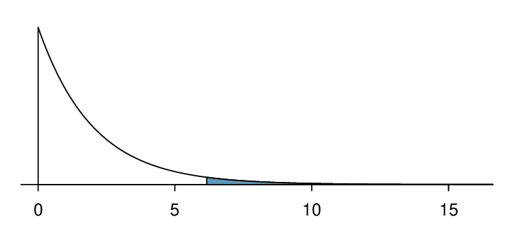
Calculate: Using technology, we get
\(\chi^2 = 91.9\text{.}\) The degrees of freedom for this test is given by:
\(df = (\# \text{ of rows } - 1) \times (\# \text{ of columns } - 1) = 3\times 1 = 3\)
The p-value is the area under the chi-square curve with 3 degrees of freedom to the right of
\(\chi^2=91.9\text{.}\) Thus, the p-value
\(=8.46\times10^{-20} \approx 0\text{.}\)
Conclude: Because the p-value
\(\approx 0 \lt \alpha\text{,}\) we reject
\(H_0\text{.}\) We have sufficient evidence that generation and taking action to help address climate change are dependent