Identify: We will test the following hypotheses at the
\(\alpha=0.05\) significance level.
\(H_0\text{:}\) \(\mu=0.25\)
\(H_A\text{:}\) \(\mu \ne 0.25\) The mean mercury content is not 0.25 ppm.
Choose: Because we are hypothesizing about a single mean we choose the 1-sample
\(t\)-test.
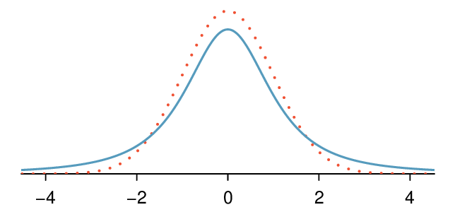
Check: The conditions were checked previously, namely — the data come from a random sample, and because
\(n\) is less than 30, we verified that there is no strong skew or outliers in the data, so the assumption that the population distribution of mercury is nearly normally distributed is reasonable.
Calculate: We will calculate the \(t\)-statistic and the p-value.
\begin{gather*}
T = \frac{\text{ point estimate } - \text{ null value } }{SE \text{ of estimate } }
\end{gather*}
The point estimate is the sample mean:
\(\bar{x}\) = 0.287
The
\(SE\) of the sample mean is:
\(\frac{s}{\sqrt{n}} = \frac{0.069}{\sqrt{15}} = 0.0178\)
The null value is the value hypothesized for the parameter in
\(H_0\text{,}\) which is 0.25.
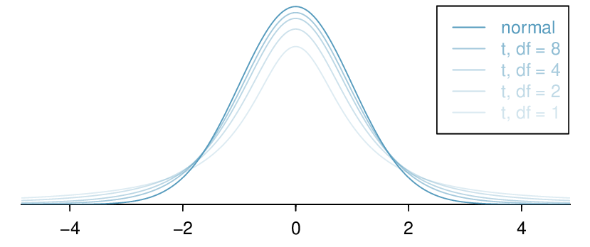
For the 1-sample \(t\)-test, \(df = n-1\text{.}\)
\begin{gather*}
T = \frac{0.287 - 0.25}{0.0178} = 2.07 \qquad df= 15-1=14
\end{gather*}
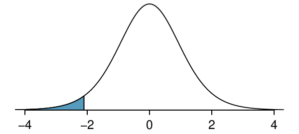
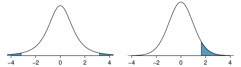
Because
\(H_A\) is a two-tailed test (
\(\ne\) ), the p-value corresponds to the area to the right of
\(t=2.07\) plus the area to the left of
\(t=-2.07\) under the
\(t\)-distribution with 14 degrees of freedom. The p-value =
\(2\times 0.029 = 0.058\text{.}\)
Conclude: The p-value of
\(0.058 > 0.05\text{,}\) so we do not reject the null hypothesis. We do not have sufficient evidence that the average mercury content in croaker white fish (Pacific) is not 0.25.