Section 10.4 Building a Single-Variable Model
As a next step we can use R to create a linear model for MCG attendance using the combined membership as the single explanatory variable using the following R code:
There are two steps here because in the first step the lm() command creates a nice big data structure full of output, and we want to hang onto that in the variable called "model1." In the second command we request an overview of the contents of model1.
It is important to note that in this model, and in the others that follow, we have added a ’-1’ term to the specification, which forces the line of best fit to pass through zero on the y-axis at zero on the x-axis (more technically speaking, the y-intercept is forced to be at the origin). In the present model that is essentially saying that if the two teams are so unpopular they don’t have any members, no one will go to see their matches, and vice versa. This technique is appropriate in this particular example, because both of the measures have sensible zero points, and we can logically reason that zero on X implies zero on Y. In most other models, particularly for survey data that may not have a sensible zero point (think about rating scales ranging from 1 to 5), it would not be appropriate to force the best fitting line through the origin.
The second command above, summary(model1), provides the following output:
    Call:

    lm(formula = MCG ~ Members 1)

    Residuals:

    Min 1Q Median 3Q Max

    -44.961 -6.550 2.954 9.931 29.252

    Coefficients:

    Estimate Std. Error t value Pr(>|t|)

    Members 1.53610 0.08768 17.52 <2e-16 ***

    --

    Signif. codes: 0 '***' 0.001 '**'' 0.01 '*'' 0.05 ''.'' 0.1 '' '' 1

    Residual standard error: 15.65 on 40 degrees of freedom

    Multiple R-squared: 0.8847,

    Adjusted R-squared: 0.8818

    F-statistic: 306.9 on 1 and 40 DF, p-value: < 2.2e-16
Wow! That’s a lot of information that R has provided for us, and we need to use this information to decide whether we are happy with this model. Being ’happy’ with the model can involve many factors, and there is no simple way of deciding. To start with, we will look at the r-squared value, also known as the coefficient of determination.
The r squared value - the coefficient of determination - represents the proportion of the variation which is accounted for in the dependent variable by the whole set of independent variables (in this case just one independent variable). An r-squared value of 1.0 would mean that the X variable(s), the independent variable(s), perfectly predicted the y, or dependent variable. An r-squared value of zero would indicated that the x variable(s) did not predict the y variable at all. R-squared cannot be negative. The r-squared of .8847 in this example means that the Combined Members variable account for 88.47% of the MCG attendance variable, an excellent result. Note that there is no absolute rule for what makes an rsquared good. Much depends on the purpose of the analysis. In the analysis of human behavior, which is notoriously unpredictable, an r-squared of .20 or .30 may be very good.
In the figure below, we have added a line of best fit based on the model to the x-y plot of MCG attendance against total team membership with this command:
> abline(model1)
While the line of best fit seems to fit the points in the middle, the points on the lower right hand side and also some points towards the top of the graph, appear to be a long way from the line of best fit. 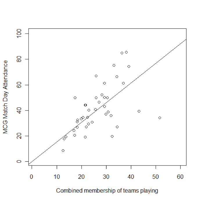
You have attempted of activities on this page.
