Introduction to Data Science Using R Runestone Version 1

Now we are ready to tackle the data.frame. In R, a data.frame is a list of columns, where each element in the list is a vector. Each vector is the same length, which is how we get our nice rectangular row and column setup, and generally each vector also has its own name. The command to make a data frame is very simple:

myFam <- data.frame(myFamName, +
myFamAge, myFamGend, myFamWeight)

Look out! We’re starting to get commands that are long enough that they break onto more than one line. The + at the end of the first line tells R to wait for more input on the next line before trying to process the command. If you want to, you can type the whole thing as one line in R, but if you do, just leave out the plus sign. Anyway, the data.frame() function makes a dataframe from the four vectors that we previously typed in. Notice that we have also used the assignment arrow to make a new stored location where R puts the data frame. This new data object, called myFam, is our dataframe. Once you have gotten that command to work, type myFam at the command line to get a report back of what the data frame contains. Here’s the output you should see:

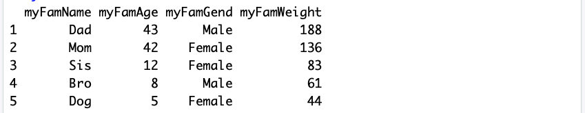
This looks great. Notice that R has put row numbers in front of each row of our data. These are different from the output line numbers we saw in brackets before, because these are actual "indices" into the data frame. In other words, they are the row numbers that R uses to keep track of which row a particular piece of data is in.

With a small data set like this one, only five rows, it is pretty easy just to take a look at all of the data. But when we get to a bigger data set this won’t be practical. We need to have other ways of summarizing what we have. R’s str() method stands for structure and compactly reveals the type of "structure" that R has used to store a data object.

Take note that for the first time, the example shows the command prompt ">" in order to differentiate the command from the output that follows. You don’t need to type this: R provides it whenever it is ready to receive new input. From now on in the book, there will be examples of R commands and output that are mixed together, so always be on the lookout for ">" because the command after that is what you have to type.

OK, so the function "str()" reveals the structure of the data object that you name between the parentheses. In this case we pretty well knew that myFam was a data frame because we just set that up in a previous command. In the future, however, we will run into many situations where we are not sure how R has created a data object, so it is important to know str() so that you can ask R to report what an object is at any time.

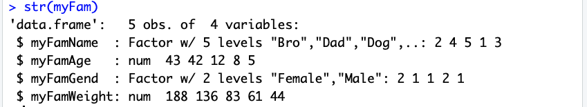
In the first line of output we have the confirmation that myFam is a data frame as well as an indication that there are five observations ("obs." which is another word that statisticians use instead of cases or instances) and four variables. After that first line of output, we have four sections that each begin with "$". For each of the four variables, these sections describe the component columns of the myFam dataframe object.

Each of the four variables has a "mode" or type that is reported by R right after the colon on the line that names the variable:

$ myFamGend : Factor w/ 2 levels

For example, myFamGend is shown as a Factor. In the terminology that R uses, "Factor" refers to a special type of label that can be used to identify and organize groups of cases. R has organized these labels alphabetically and then listed out the first few cases (because our dataframe is so small it actually is showing us all of the cases). For myFamGend we see that there are two "levels," meaning that there are two different options: female and male.

R assigns a number, starting with one, to each of these levels, so every case that is "Female" gets assigned a 1 and every case that is "Male" gets assigned a 2 (because Female comes before Male in the alphabet, so Female is the first Factor label, so it gets a 1). If you have your thinking cap on, you may be wondering why we started out by typing in small strings of text, like "Male," but then R has gone ahead and converted these small pieces of text into numbers that it calls "Factors." The reason for this lies in the statistical origins of R. For years, researchers have done things like calling an experimental group "Exp" and a control group "Ctl" without intending to use these small strings of text for anything other than labels. So R assumes, unless you tell it otherwise, that when you type in a short string like "Male" that you are referring to the label of a group, and that R should prepare for the use of Male as a "Level" of a "Factor." When you don’t want this to happen you can instruct R to stop doing this with an option on the data.frame() function: stringsAsFactors=FALSE. We will look with more detail at options and defaults a little later on.

Phew, that was complicated! By contrast, our two numeric variables, myFamAge and myFamWeight, are very simple. You can see that after the colon the mode is shown as "num" (which stands for numeric) and that the first few values are reported:

$ myFamAge : num 43 42 12 8 5

Putting it all together, we have pretty complete information about the myFam dataframe and we are just about ready to do some more work with it. We have seen firsthand that R has some pretty cryptic labels for things as well as some obscure strategies for converting this to that. R was designed for experts, rather than novices, so we will just have to take our lumps so that one day we can be experts too.