Introduction to Data Science Using R Runestone Version 1

Now we are ready to generate our test and training sets from the original spam dataset. First we will build our training set from the first 3067 rows:

We make the new data set, called trainData, using the randomized set of indices that we created in the randIndex list, but only using the first 3067 elements of randIndex (The inner expression in square brackets, 1:cutPoint2_3, does the job of selecting the first 3067 elements. From here you should be able to imagine the command for creating the test set:

The inner expression now selects the rows from 3068 all the way up to 4601 for a total of 1534 rows. So now we have two separate data sets, representing a two-thirds training and one third test breakdown of the original data. We are now in good shape to train our support vector model. The following command generates a model based on the training data set:

Using automatic sigma estimation (sigest) for RBF or laplace kernel let’s examine this command in some detail. The first argument, "type ~ .", specifies the model we want to test. Using the word "type" in this expression means that we want to have the "type" variable (i.e., whether the message is spam or non-spam) as the outcome variable that our model predicts. The tilde character ("~") in an R expression simply separates the left hand side of the expression from the right hand side. Finally, the dot character (".") is a shorthand that tell R to us all of the other variables in the dataframe to try to predict "type."

The "data" parameter let’s us specify which dataframe to use in the analysis, In this case, we have specified that the procedure should use the trainData training set that we developed.

The next parameter is an interesting one: kernel=">rbfdot". You will remember from the earlier discussion that the kernel is the customizable part of the SVM algorithm that lets us project the low dimensional problem into higher dimensional space. In this case, the rbfdot designation refers to the "radial basis function." One simple way of thinking about the radial basis function is that if you think of a point on a regular x,y coordinate system the distance from the origin to the point is like a radius of a circle. The "dot" in the name refers to the mathematical idea of a "dot product," which is a way of multiplying vectors together to come up with a single number such as a distance value. In simplified terms, the radial basis function kernel takes the set of inputs from each row in a dataset and calculates a distance value based on the combination of the many variables in the row. The weighting of the different variables in the row is adjusted by the algorithm in order to get the maximum separation of distance between the spam cases and the non-spam cases.

The "kpar" argument refers to a variety of parameters that can be used to control the operation of the radial basis function kernel. In this case we are depending on the good will of the designers of this algorithm by specifying "automatic." The designers came up with some "heuristics" (guesses) to establish the appropriate parameters without user intervention.

The C argument refers to the so called "cost of constraints." Remember back to our example of the the white top on the green mountain? When we put the piece of cardboard (the planar separation function) through the mountain, what if we happen to get one green point on the white side or one white point on the green side? This is a kind of mistake that influences how the algorithm places the piece of cardboard. We can force these mistakes to be more or less "costly," and thus to have more influence on the position of our piece of cardboard and the margin of separation that it defines. We can get a large margin of separation but possibly with a few mistakes by specifying a small value of C. If we specify a large value of C we may possibly get fewer mistakes, but on at the cost of having the cardboard cut a very close margin between the green and white points the cardboard might get stuck into the mountain at a very weird angle just to make sure that all of the green points and white points are separated. On the other hand if we have a low value of C we will get a generalizable model, but one that makes more classification mistakes.

In the next argument, we have specified "cross=3." Cross refers to the cross validation model that the algorithm uses. In this case, our choice of the final parameter, "prob.model=TRUE," dictates that we use a so called three-fold cross validation in order to generate the probabilities associate with whether a message is or isn’t a spam message. Cross validation is important for avoiding the problem of overfitting. In theory, many of the algorithms used in data mining can be pushed to the point where they essentially memorize the input data and can perfectly replicate the outcome data in the training set. The only problem with this is that the model base don the memorization of the training data will almost never generalize to other data sets. In effect, if we push the algorithm too hard, it will become too specialized to the training data and we won’t be able to use it anywhere else. By using k-fold (in this case three fold) cross validation, we can rein in the fitting function so that it does not work so hard and so that it does creat a model that is more likely to generalize to other data.

Let’s have a look at what our output structure contains:

Most of this is technical detail that will not necessarily affect how we use the SVM output, but a few things are worth pointing out. First, the sigma parameter mentioned was estimated for us by the algorithm because we used the "automatic" option. Thank goodness for that as it would have taken a lot of experimentation to choose a reasonable value without the help of the algorithm. Next, note the large number of support vectors. These are the lists of weights that help to project the variables in each row into a higher dimensional space. The "training error" at about 2.7% is quite low. Naturally, the cross-validation error is higher, as a set of parameters never perform as well on subsequent data sets as they do with the original training set. Even so, a 7.6% cross validation error rate is pretty good for a variety of prediction purposes.

We can take a closer look at these support vectors with the following command:

The alpha() accessor reveals the values of the support vectors. Note that these are stored in a nested list, hence the need for the [[1]] expression to access the first list in the list of lists. Because the particular dataset we are using only has two classes (spam or not spam), we only need one set of support vectors. If the "type" criterion variable had more than two levels (e.g., spam, not sure, and not spam), we would need additional support vectors to be able to classify the cases into more than two groups. The histogram output reveals the range of the support vectors from 0 to 5:

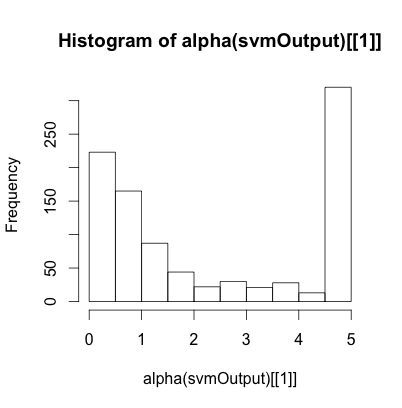
The maximum value of the support vector is equal to the cost parameter that we discussed earlier. We can see that about half of the support vectors are at this maximum value while the rest cluster around zero. Those support vectors at the maximum represent the most difficult cases to classify. WIth respect to our mountain metaphor, these are the white points that are below the piece of cardboard and the green points that are above it.

If we increase the cost parameter we can get fewer of these problem points, but at only at the cost of increasing our cross validation error:

In the first command above, the C=50 is bolded to show what we changed from the earlier command. The output here shows that our training error went way down, to 0.88%, but that our crossvalidation error went up from 7.6% in our earlier model to 8.5% in this model. We can again get a histogram of the support vectors to show what has happened:

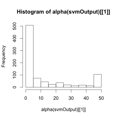
Now there are only about 100 cases where the support vector is at the maxed out value (in this case 50, because we set C=50 in the svm command). Again, these are the hard cases that the model could not get to be on the right side of the cardboard (or that were right on the cardboard). Meanwhile, the many cases with the support vector value near zero represent the combinations of parameters that make a case lie very far from the piece of cardboard. These cases were so easy to classify that they really made no contribution to "positioning" the hyperplane that separates the spam cases from the non-spam cases.

We can poke our way into this a little more deeply by looking at a couple of instructive cases. First, let’s find the index numbers of a few of the support vectors that were near zero:

This monster of a command is not as bad as it looks. We are tapping into a new part of the svmOutput object, this time using the alphaindex() accessor function. Remember that we have 850 support vectors in this output. Now imagine two lists of 850 right next to each other: the first is the list of support vectors themselves, we get at that list with the alpha() accessor function. The second list, lined right up next to the first list, is a set of indices into the original training dataset, trainData. The left hand part of the expression in the command above let’s us access these indices. The right hand part of the expression, where it says alpha(svmOutput)[[1]]<0.05, is a conditional expression that let’s us pick from the index list just those cases with a very small support vector value. You can see the output above, just underneat the command: about 15 indices were returned. Just pick off the first one, 90, and take a look at the individual case it refers to:

The command requested row 90 from the trainData training set. A few of the lines of the output were left off for ease of reading and almost all of the variables thus left out were zero. Note the very last two lines of the output, where this record is identified as a non-spam email. So this was a very easy case to classify because it has virtually none of the markers that a spam email usually has (for example, as shown above, no mention of internet, order, or mail). You can contrast this case with one of the hard cases by running this command:

You will get a list of the 92 indices of cases where the support vector was "maxed out" to the level of the cost function (remember C=50 from the latest run of the svm() command). Pick any of those cases and display it, like this:

This particular record did not have many suspicious keywords, but it did have long strings of capital letters that made it hard to classify (it was a non-spam case, by the way). You can check out a few of them to see if you can spot why each case may have been difficult for the classifier to place.