Section 10.1 The Basics of Linear Modeling

Finding relationships between sets of data is one of the key aims of data science. The question of ’does x influence y’ is of prime concern for data analysts - are house prices influenced by incomes, is the growth rate of crops improved by fertilizer, do taller sprinters run faster?
The workhorse method used by statisticians to interpret data is linear modeling, which is a term covering a wide variety of methods, from the relatively simple to very sophisticated. You can get an idea of how many different methods there are by looking at the Regression Analysis page in Wikipedia and checking out the number of entries listed under ’Models’ on the right hand sidebar (and, by the way, the list is not exhaustive).
The basis of all these methods is the idea that it is possible to fit a line to a set of data points which represents the effect an "independent" variable is having on a "dependent" variable. It is easy to visualize how this works with one variable changing in step with another variable. Figure one shows a line fitted to a series of points, using the so called "least squares" method (a relatively simple mathematical method of finding a best fitting line). Note that although the line fits the points fairly well, with an even split (as even as it can be for five points!) of points on either side of the line, none of the points are precisely on the line - the data do not fit the line precisely. As we discuss the concepts in regression analysis further, we will see that understanding these discrepancies is just as important as understanding the line itself. 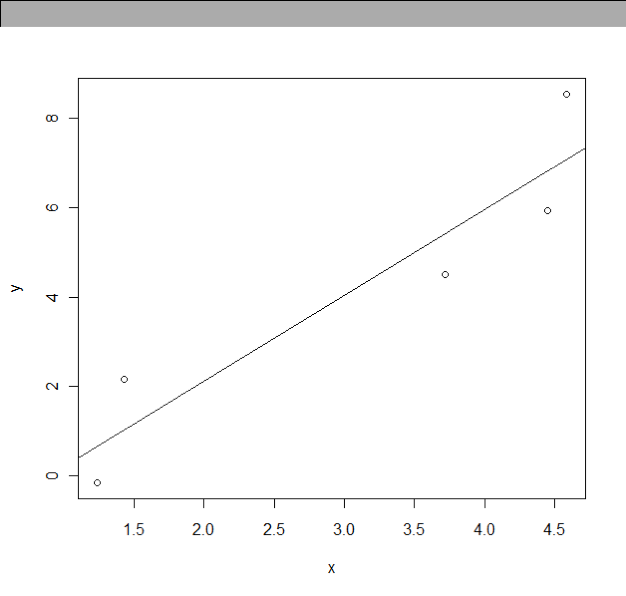
Figure: A line fitted to some points
The graph in the figure above shows how the relationship between an input variable - on the horizontal x-axis - relates to the output values on the vertical y-axis.
The original ideas behind linear regression were developed by some of the usual suspects behind many of the ideas we’ve seen already, such as Laplace, Gauss, Galton, and Pearson. The biggest individual contribution was probably by Gauss, who used the procedure to predict movements of the other planets in the solar system when they were hidden from view, and hence correctly predict when and where they would appear in view again.
The mathematical idea that allows us to fit lines of best fit to a set of data points like this is that we can find a position for the line that will minimize the distance the line is from all the points. While the mathematics behind these techniques can be handled by someone with college freshman mathematics the reality is that with even only a few data points, the process of fitting with manual calculations becomes very tedious, very quickly. For this reason, we will not discuss the specifics of how these calculations are done, but move quickly to how it can be done for us, using R.
You have attempted of activities on this page.
