Introduction to Data Science Using R Runestone Version 1

Now let’s have R calculate some statistics for us:

> var(myFam$myFamAge)

> sd(myFam$myFamAge)

Note that these commands carry on using the data used in the previous chapter, including the use of the $ to address variables within a dataframe. If you do not have the data from the previous chapter you can also do this:

> var(c(43,42,12,8,5))

> sd(c(43,42,12,8,5))

This is a pretty boring example, though, and not very useful for the rest of the chapter, so here’s the next step up in looking at data. We will use the Windows or Mac clipboard to cut and paste a larger data set into R. Go to the U.S. Census website where they have stored population data: US Census Bureau: State Population Totals: 2010-2019

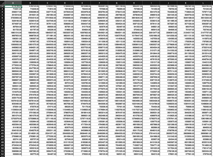
Assuming you have a spreadsheet program available, click on the XLS link for "Annual Estimates of the Resident Population for the United States, Regions, States, and Puerto Rico: April 1, 2010 to July 1, 2019 (NST-EST2019-01) " When the spreadsheet is open, select the population estimates for the fifty states. The first few looked like this in the 2011 data:

.Alabama 4,799,069

.Alaska 722,128

.Arizona 6,472,643

.Arkansas 2,940,667

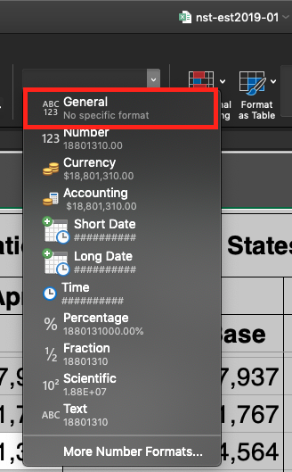
Before you copy the numbers, take out the commas by switching the cell type to "General." This can usually be accomplished under the Format menu, but you might also have a toolbar button to do the job.

Generally, you want to keep the names of columns for the data, however, for the purposes of learning just delete everything and only keep population data for the 50 states (and Washington DC). You should only have the numeric data, occupying a total of 51 lines:

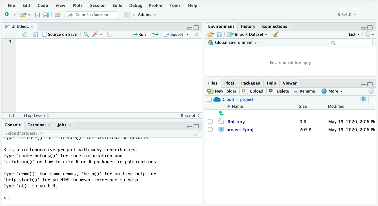
Then open R Studio Cloud and Exploring Populations Homework. In the bottom right window click on the Upload button:

Select the XSL file that you downloaded and edited and upload it. It should now appear in the Files window. Next, click on the file and select Import Dataset

You might be prompted to a page that requires installation of extensions to your Cloud environment. Click yes.

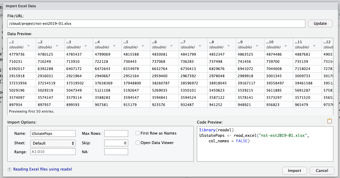
After installation of readxl and Rcpp packages for smooth integration of XSL files in our environment, you will be prompted to the Import Excel Data window. There are three changes that you will need to make 1. Change the name of the variable to which you are assigning the data from this excel sheet from its original name to USstatePops. 2. Uncheck “First Row as Names” box as we do not want the population of Alabama over different years to become the name for our columns 3. (optional) Uncheck Open Data Viewer box unless of course you are curious to see the Data Viewer window.

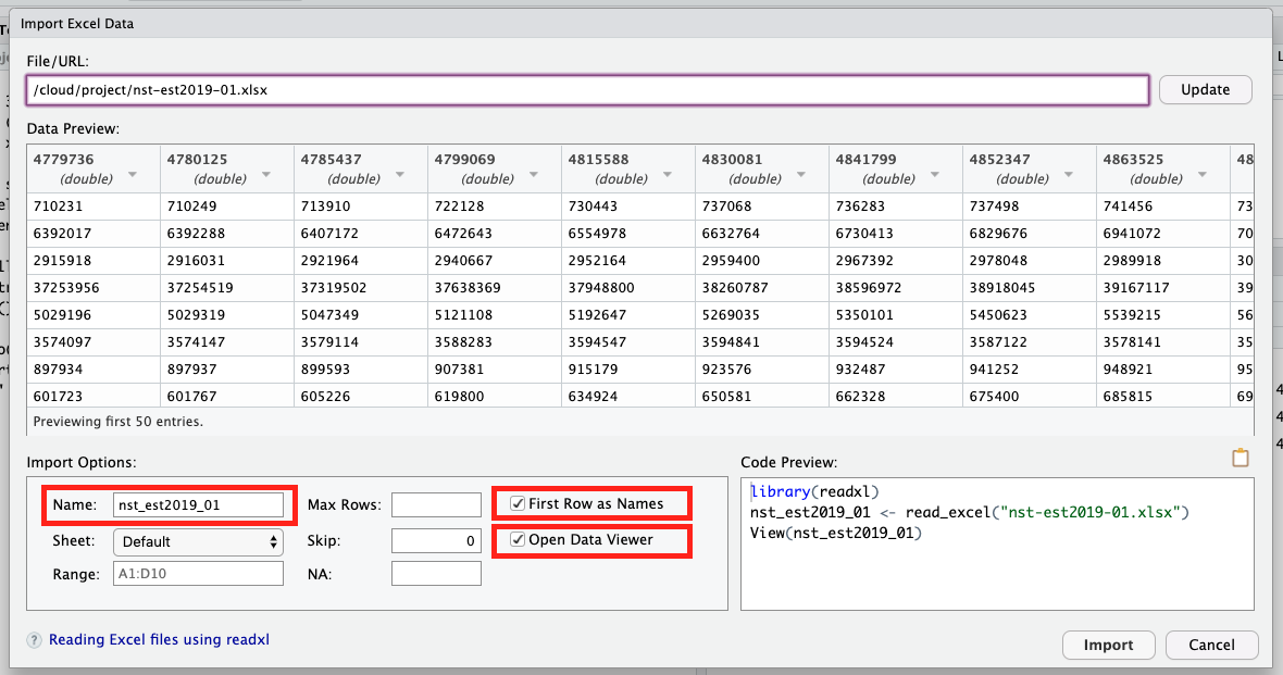
This is what the Import Excel Data window should look like after:

Nice work, you have successfully uploaded your first data set into R Studio Cloud.

Only the first three observations are shown in order to save space on this page. Your output R should show the whole list.

This would be a great moment to practice your skills from the previous chapter by using the str() and summary() functions on our new data object called USstatePops. Did you notice anything interesting from the results of these functions? One thing you might have noticed is that there are 51 observations instead of 50. Can you guess why? If not, go back and look at your original data from the spreadsheet or the U.S. Census site. The other thing you may have noticed is that USstatePops is a dataframe, and not a plain vector of numbers. You can actually see this in the output above: In the second command line where we request that R reveal what is stored in USstatePops, it responds with a column topped by the designation "V1" or “...1”. Because we did not give R any information about the numbers it read in from the clipboard, it called them "V1" or “...1”, short for Variable One, by default. So anytime we want to refer to our list of population numbers we actually have to use the name USstatePops$V1. If this sounds unfamiliar, take another look at the previous "Rows and Columns" chapter for more information on addressing the columns in a dataframe.