This section is devoted to a question that, when posed in relation to the graphs that we have examined, seems trivial. That question is: Given two vertices, \(s\) and \(t\text{,}\) of a graph, is there a path from \(s\) to \(t\text{?}\) If \(s = t\text{,}\) this question is interpreted as asking whether there is a circuit of positive length starting at \(s\text{.}\) Of course, for the graphs we have seen up to now, this question can be answered after a brief examination.
There are two situations under which a question of this kind is nontrivial. One is where the graph is very large and an “examination” of the graph could take a considerable amount of time. Anyone who has tried to solve a maze may have run into a similar problem. The second interesting situation is when we want to pose the question to a machine. If only the information on the edges between the vertices is part of the data structure for the graph, how can you put that information together to determine whether two vertices can be connected by a path?
Let \(v\) and \(w\) be vertices of a directed graph. Vertex \(v\) is connected to vertex \(w\) if there is a path from \(v\) to \(w\text{.}\) Two vertices are strongly connected if they are connected in both directions to one another. A graph is connected if, for each pair of distinct vertices, \(v\) and \(w\text{,}\)\(v\) is connected to \(w\) or \(w\) is connected to \(v\text{.}\) A graph is strongly connected if every pair of its vertices is strongly connected. For an undirected graph, in which edges can be used in either direction, the notions of strongly connected and connected are the same.
If a graph has \(n\) vertices and vertex \(u\) is connected to vertex \(w\text{,}\) then there exists a path from \(u\) to \(w\) of length no more than \(n\text{.}\)
(Indirect): Suppose \(u\) is connected to \(w\text{,}\) but the shortest path from \(u\) to \(w\) has length \(m\text{,}\) where \(m>n\text{.}\) A vertex list for a path of length \(m\) will have \(m + 1\) vertices. This path can be represented as \(\left(v_0,v_1,\ldots, v_m\right)\text{,}\) where \(v_0=u\) and \(v_m= w\text{.}\) Note that since there are only \(n\) vertices in the graph and \(m\) vertices are listed in the path after \(v_0\text{,}\) we can apply the pigeonhole principle and be assured that there must be some duplication in the last \(m\) vertices of the vertex list, which represents a circuit in the path. This means that our path of minimum length can be reduced, which is a contradiction.
Suppose that the information about edges in a graph is stored in an adjacency matrix, \(G\text{.}\) The relation, \(r\text{,}\) that \(G\) defines is \(v r w\) if there is an edge connecting \(v\) to \(w\text{.}\) Recall that the composition of \(r\) with itself, \(r^2\text{,}\) is defined by \(v r^2 w\) if there exists a vertex \(y\) such that \(v r y\) and \(y r w\text{;}\) that is, \(v\) is connected to \(w\) by a path of length 2. We could prove by induction that the relation \(r^k\text{,}\)\(k\geq 1\text{,}\) is defined by \(v r^k w\) if and only if there is a path of length \(k\) from \(v\) to \(w\text{.}\) Since the transitive closure, \(r^+\text{,}\) is the union of \(r\text{,}\)\(r^2\)\(,r^3,\ldots\text{,}\) we can answer our connectivity question by determining the transitive closure of \(r\text{,}\) which can be done most easily by keeping our relation in matrix form. Theorem 9.3.2 is significant in our calculations because it tells us that we need only go as far as \(G^n\) to determine the matrix of the transitive closure.
The main advantage of the adjacency matrix method is that the transitive closure matrix can answer all questions about the existence of paths between any vertices. If \(G^+\) is the matrix of the transitive closure, \(v_i\) is connected to \(v_j\) if and only if \(\left(G^+\right)_{i j }=1\text{.}\) A directed graph is connected if \(\left(G^+\right)_{i j }=1\) or \(\left(G^+\right)_{j i}=1\) for each \(i\neq j\text{.}\) A directed graph is strongly connected if its transitive closure matrix has no zeros.
A disadvantage of the adjacency matrix method is that the transitive closure matrix tells us whether a path exists, but not what the path is. The next algorithm will solve this problem.
The football team at Mediocre State University (MSU) has had a bad year, 2 wins and 9 losses. Thirty days after the end of the football season, the university trustees are meeting to decide whether to rehire the head coach; things look bad for him. However, on the day of the meeting, the coach issues the following press release with results from the past year:
In reality, such lists exist occasionally and have appeared in newspapers from time to time. Of course they really don’t prove anything since each team that defeated MSU in our example above can produce a similar, shorter chain of results. Since college football records are readily available, the coach could have found this list by trial and error. All that he needed to start with was that his team won at least one game. Since ESU lost one game, there was some hope of producing the chain.
The problem of finding this list is equivalent to finding a path in the tournament graph for last year’s football season that initiates at MSU and ends at ESU. Such a graph is far from complete and is likely to be represented using edge lists. To make the coach’s problem interesting, let’s imagine that only the winner of any game remembers the result of the game. The coach’s problem has now taken on the flavor of a maze. To reach ESU, he must communicate with the various teams along the path. One way that the coach could have discovered his list in time is by sending the following messages to the coaches of the two teams that MSU defeated during the season:
When this example was first written, we commented that ties should be ignored. Most recent NCAA rules call for a tiebreaker in college football and so ties are no longer an issue. Email was also not common and we described the process in terms of letters, not email messages. Another change is that the coach could also have asked the MSU math department to use Mathematica or Sage to find the path!
By making a series of phone calls, the coach can construct a path that he wants by first calling the coach who defeated ESU (the person who sent ESU’s coach that message). This coach will know who sent him a letter, and so on. Therefore, the vertex list of the desired path is constructed in reverse order.
This method could be extended to construct a list of all teams that a given team can be connected to. Simply imagine a series of letters like the one above sent by each football coach and targeted at every other coach.
The general problem of finding a path between two vertices in a graph, if one exists, can be solved exactly as we solved the problem above. The following algorithm, commonly called a breadth-first search, uses a stack.
A broadcasting algorithm for finding a path between vertex \(i\) and vertex \(j\) of a graph having \(n\) vertices. Each item \(V_k\) of a list \(V=\left\{V_1, V_2, \ldots , V_n\right\}\text{,}\) consists of a Boolean field \(V_k.\text{found}\) and an integer field \(V_k.\text{from}\text{.}\) The sets \(D_1\text{,}\)\(D_2, \dots\text{,}\) called depth sets, have the property that if \(k \in D_r\text{,}\) then the shortest path from vertex \(i\) to vertex \(k\) is of length \(r\text{.}\) In Step 5, a stack is used to put the vertex list for the path from the vertex \(i\) to vertex \(j\) in the proper order. That stack is the output of the algorithm.
If \(v_i\) is the starting vertex and we initialize \(v_i.found=False\text{,}\) then the algorithm will find the shortest circuit containing \(v_i\text{.}\) If that is of interest, we would also not initialize the depth of \(V_i\) to \(\{i\}\)
This algorithm will produce one path from vertex \(i\) to vertex \(j\text{,}\) if one exists, and that path will be as short as possible. If more than one path of this length exists, then the one that is produced depends on the order in which the edges are examined and the order in which the elements of \(D_r\) are examined in Step 4.
The condition \(D_{r }\neq \emptyset\) is analogous to the condition that no mail is sent in a given stage of the process, in which case MSU cannot be connected to ESU.
This algorithm can be easily revised to find paths to all vertices that can be reached from vertex \(i\text{.}\) Step 5 would be put off until a specific path to a vertex is needed since the information in \(V\) contains an efficient list of all paths. The algorithm can also be extended further to find paths between any two vertices.
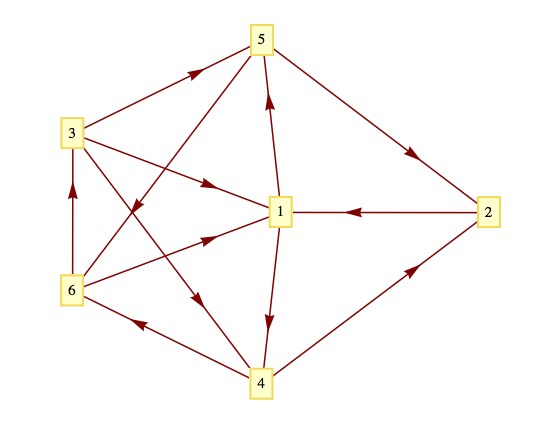
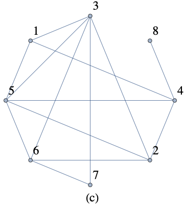
Consider the graph below. The existence of a path from vertex 2 to vertex 3 is not difficult to determine by examination. After a few seconds, you should be able to find two paths of length four. Algorithm 9.3.8 will produce one of them.
Suppose that the edges from each vertex are sorted in ascending order by terminal vertex. For example, the edges from vertex 3 would be in the order \((3, 1), (3, 4), (3, 5)\text{.}\) In addition, assume that in the body of Step 4 of the algorithm, the elements of \(D_r\) are used in ascending order. Then at the end of Step 4, the value of \(V\) will be
\begin{equation*}
\begin{array}{cccccccc}
k & 1 & 2 & 3 & 4 & 5 & 6 & \\
V_k.\text{found} & T & T & T & T & T & T & \\
V_k.\text{from} & 2 & 4 & 6 & 1 & 1 & 4 & \\
\text{Depth} \text{set} & 1 & 3 & 4 & 2 & 2 & 3 & \\
\end{array}
\end{equation*}
Therefore, the path \((2, 1, 4, 6, 3)\) is produced by the algorithm. Note that if we wanted a path from 2 to 5, the information in \(V\) produces the path (2, 1, 5) since \(V_k.\text{from} = 1\) and \(V_1.\text{from} = 2\text{.}\) A shortest circuit that initiates at vertex 2 is also available by noting that \(V_2.\text{from}=4\text{,}\)\(V_4\text{.from = 1}\text{,}\) and \(V_1.\text{from} = 2\text{;}\) thus the circuit \((2, 1, 4, 2)\) is the output of the algorithm.
If we were to perform a breadth-first search from each vertex in a graph, we could proceed to determine several key measurements relating to the general connectivity of that graph. From each vertex \(v\text{,}\) the distance from \(v\) to any other vertex \(w\text{,}\)\(d(v,w)\text{,}\) is the number of edges in the shortest path from \(v\) to \(w\text{.}\) This number is also the index of the depth set to which \(w\) belongs in a breadth-first search starting at \(v\text{.}\)
\begin{equation*}
d(v,w) = i \iff w \in D_v(i)
\end{equation*}
where \(D_v\) is the family of depth sets starting at \(v\text{.}\)
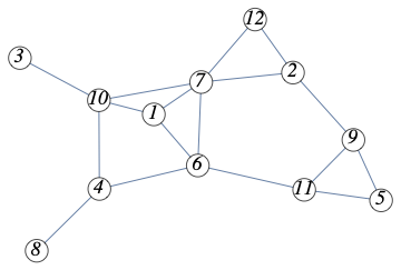
Consider Figure 9.3.13. If we perform a breadth first search of this graph starting at vertex 2, for example, we get the following “from data” telling us from what vertex each vertex is reached.
Once we know distances between any two vertices, we can determine the eccentricity of each vertex; and the graph’s diameter, radius and center. First, we define these terms precisely.
Example9.3.14.Measurements from distance matrices.
If we compute all distances between vertices, we can summarize the results in a distance matrix, where the entry in row \(i\text{,}\) column \(j\) is the distance from vertex \(i\) to vertex \(j\text{.}\) For the graph in Example 9.3.12, that matrix is
If we scan the matrix, we can see that the maximum distance is the distance between vertices 3 and 5, which is 5 and is the diameter of the graph. If we focus on individual rows and identify the maximum values, which are the eccentricities, their minimum is 3, which the graph’s radius. This eccentricity value is attained by vertices in the set \(\{1, 4, 6, 7\}\text{,}\) which is the center of the graph.
Generate a random undirected graph with 18 vertices. For each pair of vertices, an edge is included between them with probability 0.2. Since there are \(\binom{18}{2}=153\) potential edges, we expect that there will be approximately \(0.2 \cdot 153 \approx 31\) edges. The random number generation is seeded first so that the result will always be the same in spite of the random graph function. Changing or removing that first line will let you experiment with different graphs.
Generate a list of vertices that would be reached in a breadth-first search. The expression Gr.breadth_first_search(0) creates an iterator that is convenient for programming. Wrapping list( ) around the expression shows the order in which the vertices are visited with the depth set indicated in the second coordinates.
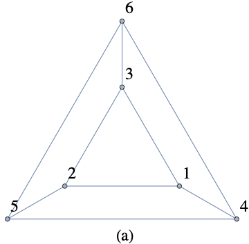
Apply Algorithm 9.3.8 to find a path from 5 to 1 in Figure 9.3.11. What would be the final value of \(V\text{?}\) Assume that the terminal vertices in edge lists and elements of the depth sets are put into ascending order, as we assumed in Example 9.3.10.
Apply Algorithm 9.3.8 to find a path from \(d\) to \(c\) in the road graph in Example 9.1.7 using the edge list in that example. Assume that the elements of the depth sets are put into ascending order.
In a simple undirected graph, what is the maximum number of edges you can have, keeping the graph unconnected? What is the minimum number of edges that will assure that the graph is connected?
If the number of vertices is \(n\text{,}\) there can be \(\frac{(n-1)(n-2)}{2}\) vertices with one vertex not connected to any of the others. One more edge and connectivity is assured.
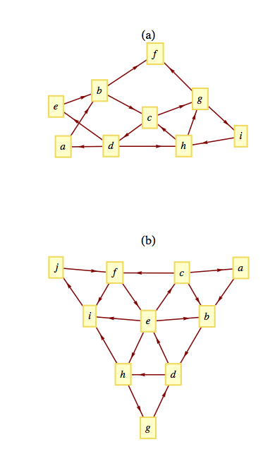
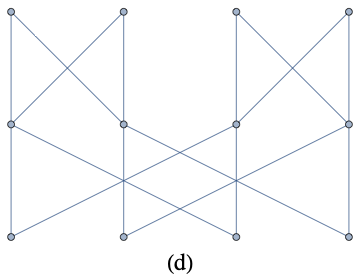
Use a broadcasting algorithm to determine the shortest path from vertex \(a\) to vertex \(i\) in the graphs shown in the Figure 9.3.15 below. List the depth sets and the stack that is created.
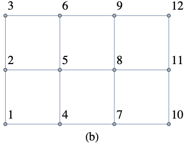
The corners (1,3,10 and 12) have eccentricities 5. The two central vertices, 5 and 8, which are in the center of the graph have eccentricity 3. All other vertices have eccentricity 4. The diameter is 5. The radius is 3.
Vertices 1, 2 and 5 have eccentricity 2 and make up the center of this graph. Verticies 7 and 8 have eccentricity 4, and all other vertices have eccentricity 3. The diameter is 4. The radius is 2.
The terms diameter, radius and center are familiar ones in the context of circles. Compare their usage in circles and graphs. How are they similar and how are they different?
Prove (by induction on \(k\)) that if the relation \(r\) on vertices of a graph is defined by \(v r w\) if there is an edge connecting \(v\) to \(w\text{,}\) then \(r^k\text{,}\)\(k \geq 1\text{,}\) is defined by \(v r^kw\) if there is a path of length \(k\) from \(v\) to \(w\text{.}\)
Basis: \((k=1)\) Is the relation \(r^1\text{,}\) defined by \(v r^1 w\) if there is a path of length 1 from \(v \text{ to } w\text{?}\) Yes, since \(v r w\) if and only if an edge, which is a path of length \(1\text{,}\) connects \(v\) to \(w\text{.}\)
Induction: Assume that \(v r^k w\) if and only if there is a path of length \(k\) from \(v\) to \(w\text{.}\) We must show that \(v r^{k+1} w\) if and only if there is a path of length \(k+1\) from \(v\) to \(w\text{.}\)
\begin{equation*}
v r^{k+1} w \Rightarrow v r^k y \textrm{ and } y r w\textrm{ for some vertex } y
\end{equation*}
By the induction hypothesis, there is a path of length \(k\) from \(v \textrm{ to } y\text{.}\) And by the basis, there is a path of length one from \(y\) to \(w\text{.}\) If we combine these two paths, we obtain a path of length \(k+1\) from \(v\) to \(w\text{.}\) Of course, if we start with a path of length \(k+1\) from \(v\) to \(w\text{,}\) we have a path of length \(k\) from \(v\) to some vertex \(y\) and a path of length 1 from \(y\) to \(w\text{.}\) Therefore, \(v r^k y \textrm{ and } y r w \Rightarrow v r^{k+1} w\text{.}\)
For each of the following distance matrices of graphs, identify the diameter, radius and center. Assume the graphs vertices are the numbers 1 through \(n\) for an \(n \times n\) matrix.
By the definition of radius, \(r\text{,}\) and diameter, \(d\text{,}\) of a connected undirected graph, we have \(r\leq d\text{.}\) Prove the upper bound on \(d\text{,}\)\(d\leq 2r\text{.}\)
Let \(v\) and \(w\) be any two vertices in the graph and let \(z\) be any vertex in the center of the graph. The distances from \(z\) to both \(v\) and \(w\) must bot be less than or equal to \(r\text{,}\) therefore, a path from \(v\) to \(w\) through \(z\) must exist and have length less than or equal to \(2r\text{.}\) Therefore \(2r\) serves as an upper bound of the diameter.