A node is a fundamental part of a tree. It can have a name, which we call the “key.” A node may also have additional information. We call this additional information the “payload.” While the payload information is not central to many tree algorithms, it is often critical in applications that make use of trees.
An edge is another fundamental part of a tree. An edge connects two nodes to show that there is a relationship between them. Every node (except the root) is connected by exactly one incoming edge from another node. Each node may have several outgoing edges.
A path is an ordered list of nodes that are connected by edges. For example, Mammal \(\rightarrow\) Carnivora \(\rightarrow\) Felidae \(\rightarrow\) Felis \(\rightarrow\) Domestica is a path.
The set of nodes \(c\) that have incoming edges from the same node to are said to be the children of that node. In Figure 8.2.2, nodes log/, spool/, and yp/ are the children of node var/.
The level of a node \(n\) is the number of edges on the path from the root node to \(n\text{.}\) For example, the level of the Felis node in Figure 8.2.1 is five. By definition, the level of the root node is zero.
With the basic vocabulary now defined, we can move on to a formal definition of a tree. In fact, we will provide two definitions of a tree. One definition involves nodes and edges. The second definition, which will prove to be very useful, is a recursive definition.
Every node \(n\text{,}\) except the root node, is connected by an edge from exactly one other node \(p\text{,}\) where \(p\) is the parent of \(n\text{.}\)
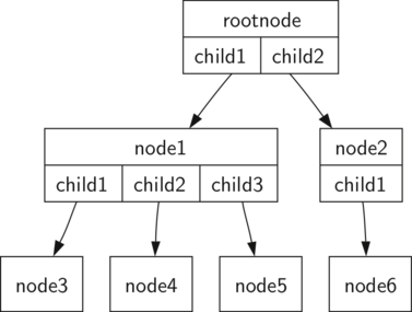
The image shows a basic conceptual diagram of a tree data structure, consisting of a set of nodes connected by edges. The top of the tree features a ’rootnode’, which branches into ’child1’ and ’child2’. Below ’child1’, there is ’node1’ with three children labeled ’child1’, ’child2’, and ’child3’, while ’child2’ branches into ’node2’ with a single ’child1’. Further down, ’node1’ branches into ’node3’, ’node4’, and ’node5’, and ’node2’ branches into ’node6’. The nodes are represented by rectangles, and the connecting lines represent the edges of the tree.
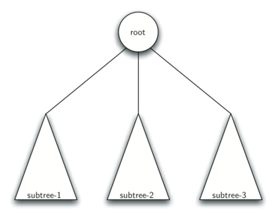
Definition Two: A tree is either empty or consists of a root and zero or more subtrees, each of which is also a tree. The root of each subtree is connected to the root of the parent tree by an edge. Figure 8.3.2 illustrates this recursive definition of a tree. Using the recursive definition of a tree, we know that the tree in Figure 8.3.2 has at least four nodes, since each of the triangles representing a subtree must have a root. It may have many more nodes than that, but we do not know unless we look deeper into the tree.
The image presents a simplified diagram of a tree data structure with a single ’root’ node at the top, branching out into three ’subtrees’ labeled ’subtree-1’, ’subtree-2’, and ’subtree-3’. This visual model illustrates the concept of recursion in data structures, where each subtree can be seen as a smaller instance of the larger structure.