Problem Solving with Algorithms and Data Structures using Python The Interactive Edition

The designers of Python had many choices to make when they implemented the list data structure. Each of these choices could have an impact on how fast list operations perform. To help them make the right choices they looked at the ways that people would most commonly use the list data structure, and they optimized their implementation of a list so that the most common operations were very fast. Of course they also tried to make the less common operations fast, but when a trade-off had to be made the performance of a less common operation was often sacrificed in favor of the more common operation.

Two common operations are indexing and assigning to an index position. Both of these operations take the same amount of time no matter how large the list becomes. When an operation like this is independent of the size of the list, it is $O(1)\text{.}$

Another very common programming task is to grow a list. There are two ways to create a longer list. You can use the append method or the concatenation operator. The append method is $O(1)\text{.}$ However, the concatenation operator is $O(k)$ where $k$ is the size of the list that is being concatenated. This is important for you to know because it can help you make your own programs more efficient by choosing the right tool for the job.

Let’s look at four different ways we might generate a list of n numbers starting with 0. First we’ll try a for loop and create the list by concatenation, then we’ll use append rather than concatenation. Next, we’ll try creating the list using list comprehension and finally, and perhaps the most obvious way, using the range function wrapped by a call to the list constructor. Listing 2.6.1 shows the code for making our list four different ways.

To capture the time it takes for each of our functions to execute we will use Python’s timeit module. The timeit module is designed to allow Python developers to make cross-platform timing measurements by running functions in a consistent environment and using timing mechanisms that are as similar as possible across operating systems.

To use timeit you create a Timer object whose parameters are two Python statements. The first parameter is a Python statement that you want to time; the second parameter is a statement that will run once to set up the test. The timeit module will then time how long it takes to execute the statement some number of times. By default timeit will try to run the statement one million times. When it’s done it returns the time as a floating-point value representing the total number of seconds. However, since it executes the statement a million times, you can read the result as the number of microseconds to execute the test one time. You can also pass timeit a named parameter called number that allows you to specify how many times the test statement is executed. The following session shows how long it takes to run each of our test functions a thousand times.

from timeit import Timer


t1 = Timer("test1()", "from __main__ import test1")
print(f"concatenation: {t1.timeit(number=1000):15.2f} milliseconds")
t2 = Timer("test2()", "from __main__ import test2")
print(f"appending: {t2.timeit(number=1000):19.2f} milliseconds")
t3 = Timer("test3()", "from __main__ import test3")
print(f"list comprehension: {t3.timeit(number=1000):10.2f} milliseconds")
t4 = Timer("test4()", "from __main__ import test4")
print(f"list range: {t4.timeit(number=1000):18.2f} milliseconds")

concatenation:           6.54 milliseconds
appending:               0.31 milliseconds
list comprehension:      0.15 milliseconds
list range:              0.07 milliseconds

In the experiment above the statement that we are timing is the function call to test1(), test2(), and so on. The setup statement may look very strange to you, so let’s consider it in more detail. You are probably very familiar with the from...import statement, but this is usually used at the beginning of a Python program file. In this case the statement from __main__ import test1 imports the function test1 from the __main__ namespace into the namespace that timeit sets up for the timing experiment. The timeit module does this because it wants to run the timing tests in an environment that is uncluttered by any stray variables you may have created that may interfere with your function’s performance in some unforeseen way.

From the experiment above it is clear that the append operation at 0.31 milliseconds is much faster than concatenation at 6.54 milliseconds. We also show the times for two additional methods for creating a list: using the list constructor with a call to range and a list comprehension. It is interesting to note that the list comprehension is twice as fast as a for loop with an append operation.

One final observation about this little experiment is that all of the times that you see above include some overhead for actually calling the test function, but we can assume that the function call overhead is identical in all four cases so we still get a meaningful comparison of the operations. So it would not be accurate to say that the concatenation operation takes 6.54 milliseconds but rather the concatenation test function takes 6.54 milliseconds. As an exercise you could test the time it takes to call an empty function and subtract that from the numbers above.

Now that we have seen how performance can be measured concretely, you can look at Table 2.6.2 to see the Big O efficiency of all the basic list operations. After thinking carefully about Table 2.6.2, you may be wondering about the two different times for pop. When pop is called on the end of the list it takes $O(1)\text{,}$ but when pop is called on the first element in the list—or anywhere in the middle it—is $O(n)$ The reason for this lies in how Python chooses to implement lists. When an item is taken from the front of the list, all the other elements in the list are shifted one position closer to the beginning. This may seem silly to you now, but if you look at Table 2.6.2 you will see that this implementation also allows the index operation to be $O(1)\text{.}$ This is a tradeoff that the Python designers thought was a good one.

As a way of demonstrating this difference in performance, let’s do another experiment using the timeit module. Our goal is to be able to verify the performance of the pop operation on a list of a known size when the program pops from the end of the list, and again when the program pops from the beginning of the list. We will also want to measure this time for lists of different sizes. What we would expect to see is that the time required to pop from the end of the list will stay constant even as the list grows in size, while the time to pop from the beginning of the list will continue to increase as the list grows.

Listing 2.6.3 shows one attempt to measure the difference between the two uses of pop. As you can see from this first example, popping from the end takes 0.00014 milliseconds, whereas popping from the beginning takes 2.09779 milliseconds. For a list of two million elements this is a factor of 15,000.

There are a couple of things to notice about Listing 2.6.3. The first is the statement from __main__ import x. Although we did not define a function, we do want to be able to use the list object x in our test. This approach allows us to time just the single pop statement and get the most accurate measure of the time for that single operation. Because the timer repeats a thousand times, it is also important to point out that the list is decreasing in size by one each time through the loop. But since the initial list is two million elements in size, we only reduce the overall size by $0.05\mathrm{\%}\text{.}$

While our first test does show that pop(0) is indeed slower than pop(), it does not validate the claim that pop(0) is $O(n)$ while pop() is $O(1)\text{.}$ To validate that claim we need to look at the performance of both calls over a range of list sizes. Listing 2.6.4 implements this test.

Figure 2.6.5 shows the results of our experiment. You can see that as the list gets longer and longer the time it takes to pop(0) also increases while the time for pop stays very flat. This is exactly what we would expect to see for an 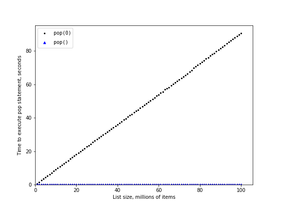$O(n)$ and $O(1)$ algorithm.

Among the sources of error in our little experiment is the fact that there are other processes running on the computer as we measure that may slow down our code, so even though we try to minimize other things happening on the computer there is bound to be some variation in time. That is why the loop runs the test one thousand times in the first place to statistically gather enough information to make the measurement reliable.