Int-Alg Answers to Selected Exercises

Appendix C Answers to Selected Exercises

1 Linear Models
1.1 Creating a Linear Model
1.1.3 Problem Set 1.1

Warm Up

1.1.3.1.

Answer.

$5.5$
🔗

🔗
$12$
🔗

🔗

🔗

1.1.3.3.

Answer.

I = 200 + 0.09 S

🔗

Skills Practice

1.1.3.5.

Answer.

\frac{6}{5}

🔗

1.1.3.7.

Answer.

y > \frac{6}{5}

🔗

1.1.3.9.

Answer.

R = 50 - 0.4 w

🔗

Applications

1.1.3.11.

Answer.

$t$ (days) $0$ $5$ $10$ $15$ $20$

$h$ (inches) 6 16 26 36 46

🔗
$h = 6 + 2 t$
🔗

🔗
$grid$

🔗
48 in
🔗

🔗
33 days
🔗

🔗
$h = 6 + 2 (21);$ $72 = 6 + 2 t$
🔗

🔗
14 is the initial height of the plants in inches. 1.5 is the number of inches they grow each day.
🔗

🔗

🔗

1.1.3.13.

Answer.

Altitude (1000 ft) $0$ $1$ $2$ $3$ $4$ $5$

Boiling point ( $^{\circ}$ F) $212$ $210$ $208$ $206$ $204$ $202$

🔗
$boiling point$

🔗
$4^{\circ}$ F

🔗
Over 4000 feet

🔗

🔗

1.2 Graphs and Equations
1.2.6 Problem Set 1.2

Warm Up

1.2.6.1.

Answer.

no

🔗
yes

🔗
no

🔗
no

🔗

🔗

1.2.6.3.

Answer.

yes

🔗
no

🔗
no

🔗
yes

🔗

🔗

1.2.6.5.

Answer.

no

🔗
no

🔗
yes

🔗
yes

🔗

🔗

1.2.6.7.

Answer.

horizontal: 0.25; vertical: 4

🔗

1.2.6.9.

Answer.

horizontal: 5; vertical: 250

🔗
$points on grid$

🔗

🔗

Skills Practice

1.2.6.11.

Answer.

\frac{- 15}{4}

🔗

1.2.6.13.

Answer.

35

🔗

1.2.6.17.

Answer.

x \geq \frac{7}{2}

🔗

$number line$

🔗

1.2.6.19.

Answer.

y = \frac{2 x}{3} + 24

🔗

1.2.6.21.

Answer.

y = \frac{- 7}{13} x + 7

🔗

1.2.6.23.

Answer.

y = \frac{2}{9} x + 17

🔗

Applications

1.2.6.25.

Answer.

1. $x = - 6$
  🔗
  
  🔗
2. $x < - 6$
  🔗
  
  🔗
3. $x > - 6$
  🔗
  
  🔗
🔗
🔗
1. $x = - 6$
  🔗
  
  🔗
2. $x < - 6$
  🔗
  
  🔗
3. $x > - 6$
  🔗
  
  🔗
🔗
🔗

🔗

1.2.6.27.

Answer.

$x = 0.3$
🔗

🔗
$x = 0.8$
🔗

🔗
$x \leq 0.3$
🔗

🔗
$x \geq 0.8$
🔗

🔗

🔗

1.2.6.29.

Answer.

$x \leq 4$
🔗

🔗
$x > 2$
🔗

🔗

🔗

1.2.6.31.

Answer.

$x = 4$
🔗

🔗
$x < 22$
🔗

🔗

🔗

1.2.6.33.

Answer.

$p = 120 + 5 t$

🔗
$increasing blood pressure$

🔗
141

🔗
7.5 min

🔗

🔗

1.3 Intercepts
1.3.6 Problem Set 1.3

Warm Up

1.3.6.1.

Answer.

$5 x$
🔗

🔗
$2 y$
🔗

🔗
5x+2y=1000
🔗

🔗

🔗

1.3.6.3.

Answer.

y = \frac{- 3}{5} x + \frac{16}{5}

🔗

Skills Practice

1.3.6.5.

Answer.

$(4, 0),$ $(0, - 3)$
🔗

🔗
$line with positive intercepts$

🔗

🔗

1.3.6.7.

Answer.

$(- 8, 0),$ $(0, 5)$
🔗

🔗
$line with positive intercepts$

🔗

🔗

1.3.6.9.

Answer.

$(3, 0), (0, 5)$
🔗

🔗
$(\frac{1}{2}, 0), (0, \frac{- 1}{4})$
🔗

🔗
$(\frac{5}{2}, 0), (0, \frac{- 3}{2})$
🔗

🔗
$(p, 0), (0, q)$
🔗

🔗
The value of $a$ is the $x$ -intercept, and the value of $b$ is the $y$ -intercept.
🔗

🔗

🔗

1.3.6.11.

Answer.

$(0, b)$
🔗

🔗
$(\frac{- b}{m}, 0)$
🔗

🔗

🔗

1.3.6.13.

Answer.

- 2 x + 3 y = 2400

🔗

1.3.6.15.

Answer.

3 x + 400 y = 240

🔗

1.3.6.17.

Answer.

$22 x + 9 y = 33,$ and

🔗
$y = \frac{11}{3} + \frac{- 22}{9} x$

🔗

🔗

1.3.6.19.

Answer.

$4 x + 12 y = 48,$ and

🔗
$y = 4 - \frac{1}{3} x$

🔗

🔗

Applications

1.3.6.21.

Answer.

$9 x$
🔗

🔗
$4 y$
🔗

🔗
$9 x + 4 y = 1800$
🔗

🔗
$(200, 0)$ Delbert must eat 200g of figs daily if he eats no bananas.
🔗

🔗
$(0, 450)$ Delbert must eat 450g of bananas daily if he eats no figs.
🔗

🔗

🔗

1.3.6.23.

Answer.

$t$ $0$ $5$ $10$ $15$ $20$

$h$ $- 400$ $- 300$ $- 200$ $- 100$ $0$

🔗
$h = - 44 + 20 t$
🔗

🔗
$grid$

🔗
$(0, - 400) :$ The diver starts at a depth of 400 feet. $(20, 0) :$ The diver surfaces after 20 minutes.
🔗

🔗

🔗

1.3.6.25.

Answer.

$ $2.40 x,$ $ $3.20 y$
🔗

🔗
$2.40 x + 3.20 y = 19, 200$
🔗

🔗
🔗
The $y$ -intercept, 6000 gallons, is the amount of premium that the gas station owner can buy if he buys no regular. The $x$ -intercept, 8000 gallons, is the amount of regular he can buy if he buys no premium.
🔗

🔗

🔗

1.4 Slope
1.4.5 Problem Set 1.4

Warm Up

1.4.5.1.

Answer.

Anthony

🔗

1.4.5.3.

Answer.

Bob’s driveway

🔗

1.4.5.5.

Answer.

- 1

🔗

1.4.5.7.

Answer.

\frac{- 2}{3}

🔗

Skills Practice

1.4.5.9.

Answer.

$\frac{3}{2}$

🔗
$6, \frac{3}{2}$

🔗
$- 9, \frac{3}{2}$

🔗
27

🔗

🔗

1.4.5.11.

Answer.

\frac{3}{4}

🔗

1.4.5.13.

Answer.

- 4000

🔗

1.4.5.15.

Answer.

$9x+12y=36$

🔗
$m = \frac{- 3}{4}$

🔗

🔗

1.4.5.17.

Answer.

14.29 ft

🔗

1.4.5.19.

Answer.

(a)

🔗

Applications

1.4.5.21.

Answer.

$del x and del y$

🔗
800

🔗
$P = 7000 + 800 t$

🔗

🔗

1.4.5.23.

Answer.

$- 6$ liters/day
🔗

🔗
The water supply is decreasing at a rate of 6 liters per day.
🔗

🔗
$line with changes in W and t$

🔗
$W = 48 - 6 t$
🔗

🔗

🔗

1.4.5.25.

Answer.

Yes, the slope is 0.12
🔗

🔗
0.12 cm/kg: The spring stretches an extra 0.12 cm for each additional 1 kg mass.
🔗

🔗

🔗

1.4.5.27.

Answer.

The distances to the stations are known.

🔗
5.7 km/sec

🔗

🔗

1.4.5.29.

Answer.

7.9

🔗
8.35 km

🔗
2 hrs 5 min

🔗

🔗

1.5 Equations of Lines
1.5.6 Problem Set 1.5

Warm Up

1.5.6.1.

Answer.

$x$	$- 1$	$0$	$2$	$3$	$4$
$y$	$10$	$8$	$4$	$2$	$0$

$line$

8
🔗

🔗
decreases by 2 units
🔗

🔗
The constant term is the $y$ -intercept and the coefficient of $x$ is the slope.

🔗

🔗

1.5.6.3.

Answer.

$Δ h = 22$

🔗
$Δ r = - 57$

🔗

🔗

Skills Practice

1.5.6.5.

Answer.

$y = \frac{- 3}{2} x + \frac{1}{2}$

🔗
$m = \frac{- 3}{2}; b = \frac{1}{2}$

🔗

🔗

1.5.6.7.

Answer.

$y = 14 x - 22$

🔗
$m = 14; b = - 22$

🔗

🔗

1.5.6.9.

Answer.

$line$

🔗
$y = \frac{- 5}{3} x - 6$

🔗
$x = \frac{- 18}{5}$

🔗

🔗

1.5.6.11.

Answer.

II
🔗

🔗
III
🔗

🔗
I
🔗

🔗
IV
🔗

🔗

🔗

1.5.6.13.

Answer.

$line through (2,-5) with slope -3$

🔗
$y + 5 = - 3 (x - 2)$
🔗

🔗
$y = - 3 x + 1$
🔗

🔗

🔗

1.5.6.15.

Answer.

y = 4 x + 40

🔗

1.5.6.17.

Answer.

III
🔗

🔗
IV
🔗

🔗
II
🔗

🔗
I
🔗

🔗

🔗

Applications

1.5.6.19.

Answer.

$M = 7000 - 400 w$
🔗

🔗
The slope tells us that Tammy’s bank account is diminishing at a rate of $400 per week, the vertical intercept that she had $7000 (when she lost all sources of income).
🔗

🔗

🔗

1.5.6.21.

Answer.

m = - 0.0018

degree/foot, so the boiling point drops with altitude at a rate of 0.0018 degree per foot.

b = 212,

so the boiling point is

212^{\circ}

at sea level (where the elevation

h = 0

🔗

1.5.6.23.

Answer.

$h$ $8$ $20$

$C$ $645$ $1425$

🔗
$C = 125 + 65 h$
🔗

🔗
$m = 65,$ the lesson rate is 65 dollars per hour
🔗

🔗

🔗

1.5.6.25.

Answer.

$C$ $15$ $- 5$

$F$ $59$ $23$

🔗
$F = 32 + \frac{9}{5} C$
🔗

🔗
$m = \frac{9}{5},$ so an increase of $1^{\circ}$ C is equivalent to an increase of ${\frac{9}{5}}^{\circ}$ F.
🔗

🔗

🔗

1.5.6.27.

Answer.

$55^{\circ}$ F
🔗

🔗
9840 ft
🔗

🔗
$temperature vs altitude$

🔗
$m = \frac{- 3}{820} .$ The temperature decreases 3 degrees for each increase in altitude of 820 feet.
🔗

🔗
$(19, 133 \frac{1}{3}, 0) .$ At an altitude of $19, 133 \frac{1}{3}$ feet, the temperature is $0^{\circ}$ F. $(0, 70) .$ At an altitude of 0 feet, the temperature is $70^{\circ}$ F.
🔗

🔗

🔗

1.5.6.29.

Answer.

$(0, 28)$
🔗

$salt dissolved$

🔗
$m = \frac{1}{2}$
🔗

🔗
$y = \frac{1}{2} x + 28$
🔗

🔗
$36^{\circ} C$
🔗

🔗

🔗

1.6 Chapter Summary and Review
1.6.3 Chapter 1 Review Problems

1.6.3.1.

Answer.

$n$ $100$ $500$ $800$ $1200$ $1500$

$C$ $4000$ $12, 000$ $18, 000$ $26, 000$ $32, 000$

🔗
$C = 20 n + 2000$
🔗

🔗
$cost of producing calculators$

🔗
$22,000
🔗

🔗
400
🔗

🔗

🔗

1.6.3.2.

Answer.

$t$ $5$ $10$ $15$ $20$ $25$

$R$ $1960$ $1820$ $1680$ $1540$ $1400$

🔗
$R = 2100 - 28 t$
🔗

🔗
$(75, 0),$ $(0, 2100)$
🔗

$grid$

🔗
$t$ -intercept: The oil reserves will be gone in 2080; $R$ -intercept: There were $2100$ billion barrels of oil reserves in 2005.
🔗

🔗

🔗

1.6.3.3.

Answer.

$60 C + 100 T = 1200$
🔗

🔗
$(20, 0),$ $(0, 12)$
🔗

$grid$

🔗
6 days
🔗

🔗
She can spend 20 days in Atlantic City if she spends no time in Saint-Tropez, or 12 days in Saint-Tropez if she spends no time in Atlantic City.
🔗

🔗

🔗

1.6.3.4.

Answer.

$line with x-intercept 5, y-intercept -12$

🔗

1.6.3.5.

Answer.

$line with x-intercept -400, y-intercept 500$

🔗

1.6.3.6.

Answer.

$line with x-intercept 6, y-intercept 4$

🔗

1.6.3.7.

Answer.

$line through origin with slope 3/4$

🔗

1.6.3.8.

Answer.

$line through origin with slope -1/4$

🔗

1.6.3.9.

Answer.

$verticalline x= -3$

🔗

1.6.3.10.

Answer.

$B = 800 - 5 t$
🔗

🔗
🔗
$m = - 5$ thousand barrels/minute: The amount of oil in the tanker is decreasing by 5000 barrels per minute.
🔗

🔗

🔗

1.6.3.11.

Answer.

$F = 500 + 0.10 C$
🔗

🔗
🔗
$m = 0.10 :$ The fee increases by $0.10 for each dollar increase in the remodeling job.
🔗

🔗

🔗

1.6.3.12.

Answer.

\frac{- 3}{2}

🔗

1.6.3.13.

Answer.

2

🔗

1.6.3.14.

Answer.

- 0.4

🔗

1.6.3.15.

Answer.

- 1.75

🔗

1.6.3.16.

Answer.

neither

🔗

1.6.3.17.

Answer.

both

🔗

1.6.3.18.

Answer.

$d$	$V$
$- 5$	$- 4.8$
$- 2$	$- 3$
$1$	$- 1.2$
$6$	$1.8$
$10$	$4.2$

🔗

1.6.3.19.

Answer.

$q$	$S$
$- 8$	$- 8$
$- 4$	$36$
$3$	$168$
$5$	$200$
$9$	$264$

🔗

1.6.3.20.

Answer.

80 ft

🔗

1.6.3.21.

Answer.

m = \frac{1}{2},

b = \frac{- 5}{4}

🔗

1.6.3.22.

Answer.

m = \frac{3}{4},

b = \frac{5}{4}

🔗

1.6.3.23.

Answer.

m = - 4,

b = 3

🔗

1.6.3.24.

Answer.

m = 0,

b = 3

🔗

1.6.3.25.

Answer.

$line through (-4,6), slope -2/3$

🔗
$y = \frac{- 2}{3} x + \frac{10}{3}$
🔗

🔗

🔗

1.6.3.26.

Answer.

$line through (2,-5), slope 3/2$

🔗
$y = \frac{3}{2} x - 8$
🔗

🔗

🔗

1.6.3.27.

Answer.

$T = 62 - 0.0036 h$
🔗

🔗
$- 46^{\circ} F;$ $108^{\circ} F$
🔗

🔗
$- 71^{\circ} F$
🔗

🔗

🔗

1.6.3.28.

Answer.

y = \frac{- 9}{5} x + \frac{2}{5}

🔗

1.6.3.29.

Answer.

y = \frac{- 5}{2} x + 8

🔗

1.6.3.30.

Answer.

$t$ $0$ $15$

$P$ $4800$ $6780$

🔗
$P = 4800 + 132 t$
🔗

🔗
$m = 132$ people/year: the population grew at a rate of $132$ people per year.
🔗

🔗

🔗

1.6.3.31.

Answer.

$m = - 2;$ $b = 3$
🔗

🔗
$y = - 2 x + 3$
🔗

🔗

🔗

1.6.3.32.

Answer.

$m = \frac{3}{2};$ $b = - 5$
🔗

🔗
$y = \frac{3}{2} x - 5$
🔗

🔗

🔗

1.6.3.33.

Answer.

\frac{3}{5}

🔗

1.6.3.34.

Answer.

$(4, 0)$ and $(0, - 6)$
🔗

🔗
$\frac{3}{2}$
🔗

🔗

🔗

1.6.3.35.

Answer.

$(\frac{8}{3}, 0)$ and $(0, - 4)$
🔗

🔗
$(4, 3);$ No
🔗

🔗

🔗

2 Applications of Linear Models
2.1 Linear Regression
2.1.5 Problem Set 2.1

Warm Up

2.1.5.1.

Answer.

a: II; b: III; c: I; d: IV

🔗

2.1.5.2.

Answer.

a: III; b: IV; c: II; d: I

🔗

2.1.5.3.

Answer.

$k$ $70$ $50$

$p$ $154$ $110$

🔗
$p = 2.2 k$
🔗

🔗
$m = 2.2$ pounds/kg is the conversion factor from kilograms to pounds
🔗

🔗

🔗

Skills Practice

2.1.5.5.

Answer.

The slope is

- 2.5,

which indicates that the snack bar sells 2.5 fewer cups of cocoa for each

1^{\circ} C

increase in temperature. The

C

-intercept of 52 indicates that 52 cups of cocoa would be sold at a temperature of

0^{\circ} C .

The

T

-intercept of 20.8 indicates that no cocoa will be sold at a temperature of

{20.8}^{\circ} C .

🔗

2.1.5.7.

Answer.

🔗

2.1.5.9.

Answer.

$L = 24 + (29 / 7) t,$ where $t$ is in months
🔗

🔗
74 feet

🔗
The young whale grows in length about 4.14 foot per month

🔗

🔗

2.1.5.11.

Answer.

2 min:

21^{\circ}

C; 2 hr:

729^{\circ}

C; The estimate at 2 minutes is reasonable; the estimate at 2 hours is not reasonable.

🔗

Applications

2.1.5.13.

Answer.

12 seconds
🔗

🔗
39
🔗

🔗
🔗
11.6 seconds
🔗

🔗
$y = 8.5 + 0.1 x$
🔗

🔗
12.7 seconds; 10.18 seconds; The prediction for the 40-year-old is reasonable, but not the prediction for the 12-year-old.
🔗

🔗

🔗

2.1.5.15.

Answer.

🔗
53 sec, 64 sec

🔗
$y = 5.5 x - 8.6$

🔗
57.95 sec

🔗

🔗

2.1.5.17.

Answer.

🔗
$y = 121 + 19.86 t$
🔗

🔗
$419$
🔗

🔗

🔗

2.1.5.19.

Answer.

$scatterplot and regression line$

🔗
The graph is above.
🔗

🔗
The slope tells us that the time it takes for a bird to attract a mate decreases by 0.85 days for every additional song it learns.
🔗

🔗
44.5 days
🔗

🔗
The $C$ -intercept tells us that a warbler with a repretoire of 53 songs would acquire a mate immediately. The $B$ -intercept tells us that a warbler with no songs would take 62 days to find a mate. These values make sense in context.
🔗

🔗

🔗

2.2 Linear Systems
2.2.5 Problem Set 2.2

Warm Up

2.2.5.1.

Answer.

$line$

🔗

2.2.5.3.

Answer.

18.75

🔗

Skills Practice

2.2.5.5.

Answer.

(- 4, 5)

🔗

2.2.5.7.

Answer.

(- 2, 3)

🔗

2.2.5.9.

Answer.

Inconsistent

🔗

2.2.5.11.

Answer.

Dependent

🔗

Applications

2.2.5.13.

Answer.

Sporthaus: $y = 500 + 10 x$
🔗

Fitness First: $y = 50 + 25 x$
🔗

🔗
$x$ Sporthaus Fitness First

6 560 200

12 620 350

18 680 500

24 740 650

30 800 800

36 860 950

42 920 1100

48 980 1250

🔗
$Cost for fitness clubs$

🔗
30 months
🔗

🔗

🔗

2.2.5.15.

Answer.

$10 x + 5 y = 300$
🔗

🔗
$y = 3 x$
🔗

🔗
$two lines$

$(12, 36)$
🔗

🔗
She should buy 12 hardbacks and 36 paperbacks.
🔗

🔗

🔗

2.2.5.17.

Answer.

$S = 1.5 x$
🔗

🔗
$D = 120 - 2.5 x$
🔗

🔗
$two lines$

🔗
$x = 30;$ $S = 45$
🔗

🔗

🔗

2.2.5.19.

Answer.

The median age

🔗
$grid$

🔗
0.3 years of age per year since 1990

🔗
See (b) above

🔗
Slightly less than 14 years since 1990

🔗
More than half the women are older than the mean age of women.

🔗

🔗

2.3 Algebraic Solution of Systems
2.3.5 Problem Set 2.3

Warm Up

2.3.5.1.

Answer.

(4, 1)

🔗

Skills Practice

2.3.5.3.

Answer.

(1, 2)

🔗

2.3.5.7.

Answer.

(1, 2)

🔗

2.3.5.9.

Answer.

Dependent

🔗

Applications

2.3.5.11.

Answer.

$S = 2.5 x; D = 350 - 4.5 x$

🔗
50 dollars per machine; 125 machines

🔗

🔗

2.3.5.13.

Answer.

Pounds % silver Amount of silver

First alloy $x$ $0.45$ $0.45 x$

Second alloy $y$ $0.60$ $0.60 y$

Mixture $40$ $0.48$ $0.48 (40)$

🔗
$x + y = 40$
🔗

🔗
$0.45 x + 0.60 y = 19.2$
🔗

🔗
32 lb
🔗

🔗

🔗

2.3.5.15.

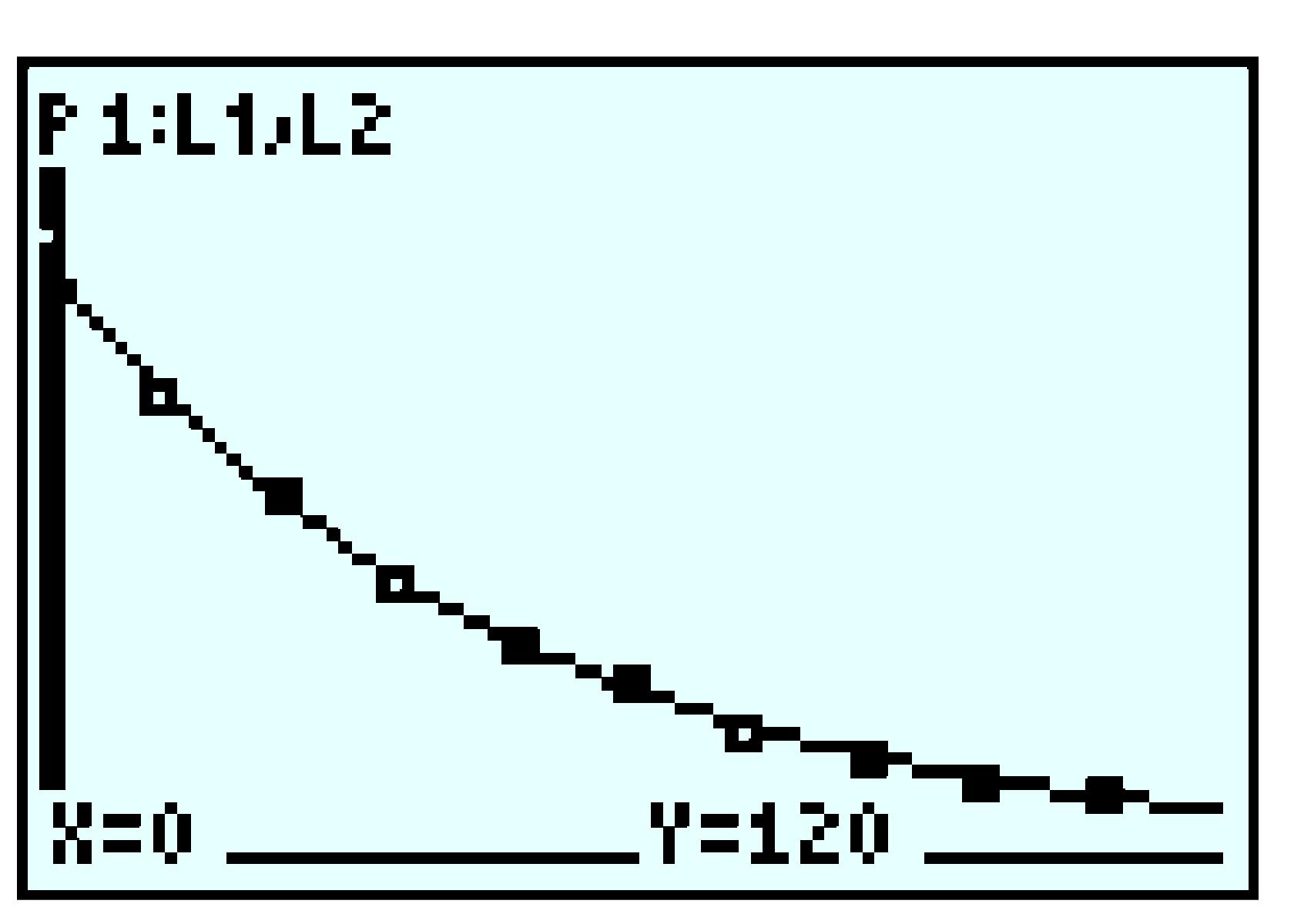
Answer.

Rani’s speed in still water: $x$

Speed of the current: $y$

Rate Time Distance

Downstream $x + y$ $45$ $6000$

Upstream $x - y$ $45$ $4800$

🔗
$45 (x + y) = 6000$
🔗

🔗
$45 (x - y) = 4800$
🔗

🔗
Rani’s speed in still water is 120 meters per minute, and the speed of the current is $13 \frac{1}{3}$ meters per minute.
🔗

🔗

🔗

2.3.5.17.

Answer.

607.5 mi

🔗

2.3.5.19.

Answer.

Sports coupes Wagons Total

Hours of riveting 3 4 120

Hours of welding 4 5 155

🔗
$3 x + 4 y = 120$

🔗
$4 x + 5 y = 155$

🔗
20 sports coupes and 15 wagons

🔗

🔗

2.4 Gaussian Reduction
2.4.6 Problem Set 2.4

Warm Up

2.4.6.1.

Answer.

(- 3, - 5)

🔗

2.4.6.3.

Answer.

Principal Interest rate Interest

Bonds $x$ $0.10$ $0.10 x$

Certificate $y$ $0.08$ $0.08 y$

Total $2000$ —— $184$

🔗
$x + y = 2000$
🔗

🔗
$0.10 x + 0.08 y = 184$
🔗

🔗

🔗

Skills Practice

2.4.6.5.

Answer.

(- 2, 0, 3)

🔗

2.4.6.7.

Answer.

(2, - 2, 0)

🔗

2.4.6.9.

Answer.

(2, - 3, 1)

🔗

2.4.6.11.

Answer.

(\frac{1}{2}, \frac{2}{3}, - 3)

🔗

2.4.6.13.

Answer.

(\frac{1}{2}, - \frac{1}{2}, \frac{1}{3})

🔗

2.4.6.15.

Answer.

Dependent

🔗

Applications

2.4.6.17.

Answer.

x = 40

in,

y = 60

in,

z = 55

🔗

2.4.6.19.

Answer.

\frac{1}{2}

lb Colombian,

\frac{1}{4}

lb French,

\frac{1}{4}

Sumatran

🔗

2.4.6.21.

Answer.

🔗

2.5 Linear Inequalities in Two Variables
2.5.5 Problem Set 2.5

Warm Up

2.5.5.1.

Answer.

$x$ $- 2$ $5$ $6$ $8$

$y$ $12$ $5$ $4$ $2$

🔗
$grid$

🔗
$x + y = 10$
🔗

🔗
See above.
🔗

🔗

🔗

2.5.5.3.

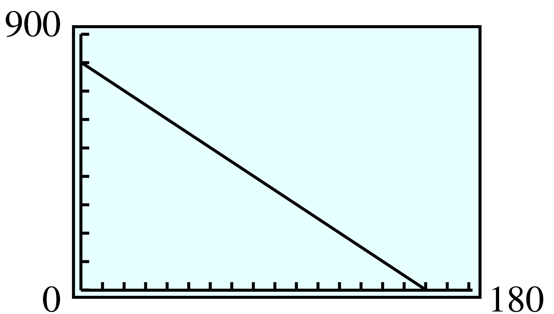
Answer.

The graph of the equation is a line, and the graph of the inequality is a half-plane. The line is the boundary of the half-plane but is not included in the solution to the inequality.
🔗

🔗
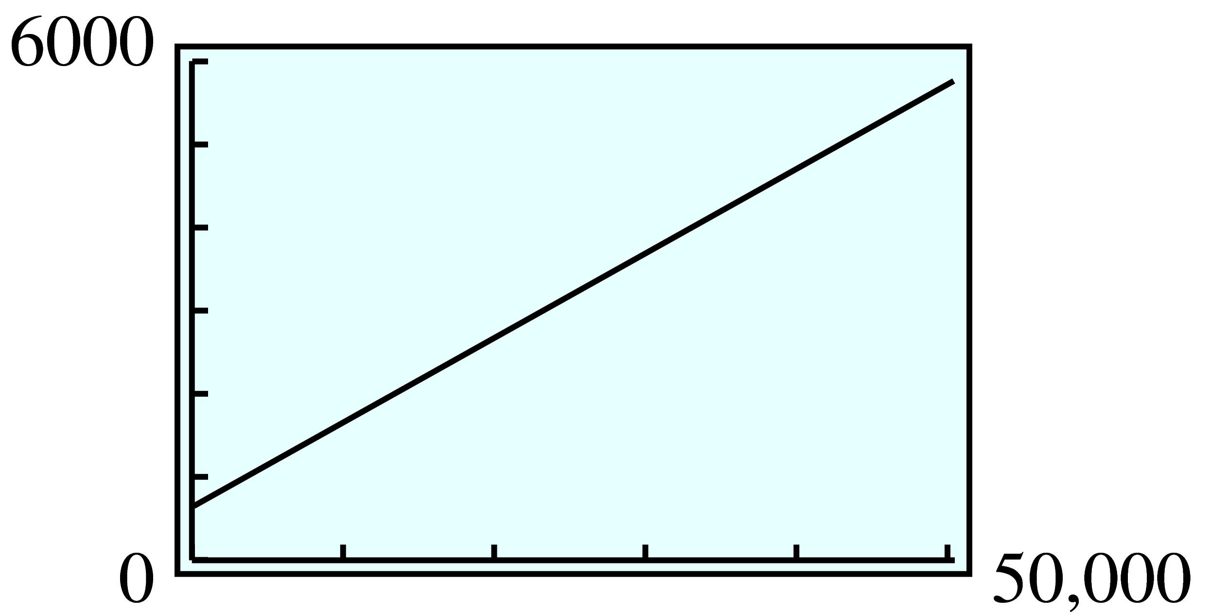
The graph of $x + y \geq 10, 000$ includes both the line $x + y = 10, 000$ and the half-plane of the corresponding strict inequality.
🔗

🔗

🔗

Skills Practice

2.5.5.5.

Answer.

🔗

2.5.5.7.

Answer.

$linear inequality in two variables$

🔗

2.5.5.9.

Answer.

🔗

2.5.5.11.

Answer.

🔗

2.5.5.13.

Answer.

🔗

2.5.5.15.

Answer.

🔗

2.5.5.17.

Answer.

🔗

2.5.5.19.

Answer.

🔗

2.5.5.21.

Answer.

🔗

2.5.5.23.

Answer.

🔗

Applications

2.5.5.25.

Answer.

🔗

2.5.5.27.

Answer.

🔗

2.6 Chapter Summary and Review
2.6.3 Chapter 2 Review Problems

2.6.3.1.

Answer.

🔗
235 kilojoules
🔗

🔗
$y = 0.106 x + 4.6$
🔗

🔗
${156.7}^{\circ} C$
🔗

🔗

🔗

2.6.3.2.

Answer.

$45$ cm
🔗

🔗
$87$ cm
🔗

🔗
$y = 1.2 x - 3$
🔗

🔗
$69$ cm
🔗

🔗
$y = 1.197 x - 3.660;$ $68.16$ cm
🔗

🔗

🔗

2.6.3.3.

Answer.

🔗

2.6.3.4.

Answer.

26 min

🔗

2.6.3.5.

Answer.

(- 1, 2)

🔗

2.6.3.6.

Answer.

(1.9, - 0.8)

🔗

2.6.3.7.

Answer.

(\frac{1}{2}, \frac{7}{2})

🔗

2.6.3.8.

Answer.

(1, 2)

🔗

2.6.3.9.

Answer.

(1, 2)

🔗

2.6.3.10.

Answer.

(\frac{1}{2}, \frac{3}{2})

🔗

2.6.3.11.

Answer.

Consistent and independent

🔗

2.6.3.12.

Answer.

Inconsistent

🔗

2.6.3.13.

Answer.

Dependent

🔗

2.6.3.14.

Answer.

Consistent and independent

🔗

2.6.3.15.

Answer.

(2, 0, - 1)

🔗

2.6.3.16.

Answer.

(2, 1, - 1)

🔗

2.6.3.17.

Answer.

(2, - 5, 3)

🔗

2.6.3.18.

Answer.

(2, \frac{3}{2}, - 1)

🔗

2.6.3.19.

Answer.

(- 2, 1, 3)

🔗

2.6.3.20.

Answer.

(2, - 1, 0)

🔗

2.6.3.21.

Answer.

🔗

2.6.3.22.

Answer.

🔗

2.6.3.23.

Answer.

$3181.82 at 8%, $1818.18 at 13.5%

🔗

2.6.3.24.

Answer.

$4000

🔗

2.6.3.25.

Answer.

5 cm, 12 cm, 13 cm

🔗

2.6.3.26.

Answer.

20 to Boston, 25 to Chicago, 10 to Los Angeles

🔗

2.6.3.27.

Answer.

$strict inequality$

🔗

2.6.3.28.

Answer.

$strict inequality$

🔗

2.6.3.29.

Answer.

$strict inequality$

🔗

2.6.3.30.

Answer.

$compound inequality$

🔗

2.6.3.31.

Answer.

$system of inequalities$

🔗

2.6.3.32.

Answer.

$system of inequalities$

🔗

2.6.3.33.

Answer.

$system of inequalities$

🔗

2.6.3.34.

Answer.

$system of inequalities$

🔗

2.6.3.35.

Answer.

$system of inequalities$

🔗

2.6.3.36.

Answer.

$system of inequalities$

🔗

2.6.3.37.

Answer.

$system of inequalities$

🔗

2.6.3.38.

Answer.

$system of inequalities$

🔗

2.6.3.39.

Answer.

20 p + 9 g \leq 120,

10 p + 10 g \leq 120,

p \geq 0,

g \geq 0

🔗

$system of inequalities$

🔗

2.6.3.40.

Answer.

x + y \leq 32,

2 x + 1.6 y \geq 56,

x \geq 0,

y \geq 0,

where

x

represents ounces of tofu,

y

the ounces of tempeh

🔗

$system of inequalities$

🔗

3 Quadratic Models
3.1 Extraction of Roots
3.1.9 Problem Set 3.1

Warm Up

3.1.9.1.

Answer.

$- 12$
🔗

🔗
$- 2$
🔗

🔗
$9$
🔗

🔗

🔗

3.1.9.3.

Answer.

$29$
🔗

🔗
$7$
🔗

🔗
$\sqrt{6}$
🔗

🔗

🔗

3.1.9.4.

Answer.

$\pm 7$
🔗

🔗
$\pm \frac{5}{2}$
🔗

🔗
$\pm \sqrt{5}$
🔗

🔗

🔗

3.1.9.5.

Answer.

$parabola$

🔗
Two solutions. $\approx \pm 2.5$

🔗
$\pm \sqrt{6}$

🔗

🔗

Skills Practice

3.1.9.7.

Answer.

\pm \sqrt{3}

🔗

3.1.9.9.

Answer.

\frac{5}{2}, \frac{- 3}{2}

🔗

3.1.9.11.

Answer.

\frac{2}{3} \pm \frac{\sqrt{5}}{3}

🔗

3.1.9.13.

Answer.

\frac{7}{8}, \pm \frac{\sqrt{8}}{8}

🔗

3.1.9.15.

Answer.

\pm 5.73

🔗

3.1.9.17.

Answer.

b. 10, -2

🔗

3.1.9.19.

Answer.

\pm \frac{F r}{m}

🔗

3.1.9.21.

Answer.

\pm p i \sqrt{\frac{L}{8}}

🔗

Applications

3.1.9.23.

Answer.

21 in

🔗

3.1.9.25.

Answer.

$A = 1600 (1 + r)^{2}$

🔗
$r$ $0.02$ $0.04$ $0.06$ $0.08$

$A$ $1664.64$ $1730.56$ $1797.76$ $1866.24$

🔗
11.8%

🔗

🔗

3.1.9.27.

Answer.

19 ft by 57 ft

🔗

3.1.9.29.

Answer.

$V = 62.8 r^{2}$

🔗
$\frac{1}{4}$

🔗
1.96 cm

🔗

🔗

3.1.9.31.

Answer.

$\pm \sqrt{\frac{b c}{a}}$

🔗
$\pm \sqrt{\frac{a c}{b}}$

🔗

🔗

3.2 Intercepts, Solutions, and Factors
3.2.6 Problem Set 3.2

Warm Up

3.2.6.1.

Answer.

$2 b^{2} + 9 b - 18$

🔗
$12 z^{2} - 35 z + 8$

🔗

🔗

3.2.6.3.

Answer.

$6 p^{3} - 33 p^{2} + 45 p$

🔗
$6 v^{3} + 16 v^{2} - 32 v$

🔗

🔗

3.2.6.5.

Answer.

$(x - 4) (x + 4)$
🔗

🔗
$x (x - 16)$
🔗

🔗
$(x - 4) (x - 4)$
🔗

🔗
cannot be factored
🔗

🔗

🔗

3.2.6.7.

Answer.

(x - 5) (x - 2)

🔗

3.2.6.9.

Answer.

(w - 8) (w + 4)

🔗

3.2.6.11.

Answer.

(x - 5) (x - 2)

🔗

Skills Practice

3.2.6.13.

Answer.

\frac{1}{2}, - 3

🔗

3.2.6.15.

Answer.

0, 3

🔗

3.2.6.17.

Answer.

\frac{1}{2}, 1

🔗

3.2.6.19.

Answer.

- 1, 2

🔗

3.2.6.21.

Answer.

\frac{7}{8} \pm \frac{\sqrt{8}}{8}

🔗

3.2.6.23.

Answer.

\frac{b \pm 5}{a}

🔗

3.2.6.25.

Answer.

0.1 (x - 18) (x + 15)

🔗

3.2.6.27.

Answer.

All three graphs have the same

x

-intercepts.

🔗

Applications

3.2.6.29.

Answer.

c. 306.5 ft at 0.625 sec d. 1.25 sec e. 5 sec

🔗

3.2.6.31.

Answer.

h^{2} + 10^{2} = (h + 2)^{2}

c. 24 ft

🔗

3.2.6.33.

Answer.

$l = x - 4, w = x - 4, h = 2, V = 2 (x - 4)^{2}$

🔗
0 cubic in, 2 cubic in, 8 cubic in, etc.

🔗
$x = 4$

🔗
9 in by 9 in

🔗
$2 (x - 4)^{2} = 50; x = 9$

🔗

🔗

3.2.6.34.

Answer.

l = 6, w = 1 - 2 x, h = x, V = 6 x (1 - 2 x)

6 x (1 - 2 x) = \frac{3}{4}; \frac{1}{4}

🔗

3.3 Graphing Parabolas
3.3.6 Problem Set 3.3

Warm Up

3.3.6.1.

Answer.

13

🔗

3.3.6.4.

Answer.

factoring; $0, 10$

🔗
extraction of roots; $\pm \sqrt{10}$

🔗
factoring; $\frac{- 1}{2}, 1$

🔗
extraction of roots; $\frac{- 5}{2}, \frac{- 5}{2}$

🔗

🔗

3.3.6.6.

Answer.

2 π R (R + H)

🔗

3.3.6.8.

Answer.

0, - 35

🔗

Skills Practice

3.3.6.9.

Answer.

ii

🔗
iv

🔗
i

🔗
iii

🔗
vi

🔗
v

🔗

🔗

3.3.6.11.

Answer.

1. Narrower
  
  🔗
2. $graph y=2x-squared$
  
  🔗
🔗
🔗
1. Wider
  
  🔗
2. $graph y=2x-squared$
  
  🔗
🔗
🔗
1. Opens downward
  
  🔗
2. $graph y=neg x-squared$
  
  🔗
🔗
🔗

🔗

3.3.6.13.

Answer.

(0, 0), (4, 0); (2, - 4)

🔗

$parabola$

🔗

3.3.6.15.

Answer.

(0, 0), (- 2, 0); (- 1, - 3)

🔗

$parabola$

🔗

3.3.6.17.

Answer.

(0, 0), (20, 0); (10, 200)

🔗

$parabola$

🔗

Applications

3.3.6.19.

Answer.

$(2000, 400)$

🔗
$(0, 0), (4000, 0)$

🔗
$parabola$

🔗
$x > 4000$

🔗

🔗

3.3.6.21.

Answer.

basic parabola

🔗
narrower

🔗
wider

🔗
narrower and reflected about $y$ -axis

🔗

🔗

3.3.6.23.

Answer.

$x$ -intercepts at 0 and 4

🔗
$x$ -intercepts at 0 and $- 4$

🔗
reflection of (a) about $y$ -axis

🔗
reflection of (b) about $y$ -axis

🔗

🔗

3.4 Completing the Square
3.4.4 Problem Set 3.4

Warm Up

3.4.4.1.

Answer.

- 4, \frac{5}{2}

🔗

3.4.4.3.

Answer.

$x^{2} + 10 x + 25$

🔗
$x^{2} - 12 x + 36$

🔗
$x^{2} - 24 x + 144$

🔗
$x^{2} + 30 x + 225$

🔗

🔗

Skills Practice

3.4.4.5.

Answer.

b and c

🔗

3.4.4.7.

Answer.

- 4, - 5

🔗

3.4.4.9.

Answer.

- 1 \pm \sqrt{\frac{5}{2}}

🔗

3.4.4.11.

Answer.

\frac{- 5}{2} \pm \sqrt{\frac{45}{4}}

🔗

3.4.4.13.

Answer.

- 5, 8

🔗

3.4.4.15.

Answer.

- 3, \frac{4}{3}

🔗

Applications

3.4.4.17.

Answer.

$(\frac{1}{4} \pm \sqrt{\frac{13}{15}}, 0)$

🔗
$(\frac{1}{4}, - 3 \frac{1}{4})$

🔗

🔗

3.4.4.19.

Answer.

$(- 2, 0), (\frac{2}{5}, 0)$

🔗
$(\frac{- 4}{5}, - 7 \frac{1}{5})$

🔗

🔗

3.4.4.21.

Answer.

$L^{2} + (L - 4)^{2} = 20^{2}$

🔗
12 in by 16 in

🔗

🔗

3.4.4.23.

Answer.

$A = \frac{1}{2} (x^{2} - y^{2})$

🔗
$A = \frac{1}{2} (x - y) (x + y)$

🔗
18 sq ft

🔗

🔗

3.4.4.25.

Answer.

$A = (x + y)^{2}$

🔗
$A = x^{2} + 2 x y + y^{2}$

🔗
🔗

🔗

3.4.4.27.

Answer.

- 1 \pm \sqrt{1 - c}

🔗

3.4.4.29.

Answer.

\frac{b}{2} \pm \frac{b^{2} - 4 c}{4}

🔗

3.4.4.31.

Answer.

\pm \sqrt{\frac{V}{2 w} - s^{2}}

🔗

3.4.4.33.

Answer.

(- 15, 0), (15, 0); (0, 255)

🔗

3.4.4.35.

Answer.

\frac{- 3 x \pm 3}{2}

🔗

3.5 Chapter 3 Summary and Review
3.5.3 Chapter 3 Review Problems

3.5.3.1.

Answer.

\pm \sqrt{2}

🔗

3.5.3.2.

Answer.

\pm \sqrt{40}

🔗

3.5.3.3.

Answer.

- 4 \pm \sqrt{20}

🔗

3.5.3.4.

Answer.

\frac{1 \pm \sqrt{15}}{7}

🔗

3.5.3.5.

Answer.

1, 4

🔗

3.5.3.6.

Answer.

11.5, 23.5

🔗

3.5.3.7.

Answer.

\frac{- 3}{2}, 2

🔗

3.5.3.8.

Answer.

2, 2

🔗

3.5.3.9.

Answer.

- 2, 3

🔗

3.5.3.10.

Answer.

- 1, 1

🔗

3.5.3.11.

Answer.

4 x^{2} - 29 x - 24 = 0

🔗

3.5.3.12.

Answer.

9 x^{2} - 30 x + 25 = 0

🔗

3.5.3.13.

Answer.

y = (x - 3) (x + 2.4)

🔗

3.5.3.14.

Answer.

y = - (x + 1.3) (x - 2)

🔗

3.5.3.15.

Answer.

Vertex: $(0, 0),$ $y$ -int: $(0, 0),$ $x$ -int: $(0, 0)$
🔗

🔗
$parabola$

🔗

🔗

3.5.3.17.

Answer.

Vertex: $(\frac{9}{2}, \frac{- 81}{4}),$ $y$ -int: $(0, 0),$ $x$ -int: $(0, 0), (9, 0)$
🔗

🔗
$parabola$

🔗

🔗

3.5.3.19.

Answer.

2 \pm \sqrt{10}

🔗

3.5.3.20.

Answer.

\frac{- 3}{2} \pm \sqrt{\frac{21}{4}}

🔗

3.5.3.21.

Answer.

\frac{3}{2} \pm \sqrt{\frac{3}{4}}

🔗

3.5.3.22.

Answer.

\frac{1}{3} \pm \sqrt{\frac{10}{9}}

🔗

3.5.3.23.

Answer.

v = \pm \sqrt{\frac{2 K}{m}}

🔗

3.5.3.24.

Answer.

b = \pm \sqrt{c^{2} - a^{2}}

🔗

3.5.3.25.

Answer.

s = \pm \sqrt{\frac{3 V}{h}}

🔗

3.5.3.26.

Answer.

r = \pm \sqrt{\frac{A}{P}} - 1

🔗

3.5.3.27.

Answer.

🔗

3.5.3.28.

Answer.

🔗

3.5.3.29.

Answer.

11%

🔗

3.5.3.30.

Answer.

8.5%

🔗

3.5.3.31.

Answer.

\sqrt{108} \approx 10.4

🔗

3.5.3.32.

Answer.

17 in

🔗

3.5.3.33.

Answer.

1 sec

🔗

3.5.3.34.

Answer.

50 ft by 150 ft

🔗

3.5.3.35.

Answer.

A_{1} = x^{2} - (\frac{1}{2} y^{2} + \frac{1}{2} y^{2}) = x^{2} - y^{2}; A_{2} = (x + y) (x - y) = x^{2} - y^{2}

🔗

3.5.3.36.

Answer.

A_{1} = π (x + y)^{2} - π x^{2} - π y^{2} = 2 π x y; A_{2} = π y (2 x) = 2 π x y

🔗

4 Applications of Quadratic Models
4.1 Quadratic Formula
4.1.6 Problem Set 4.1

Warm Up

4.1.6.1.

Answer.

$8 - 2 \sqrt{20}$

🔗
$9$

🔗

🔗

4.1.6.3.

Answer.

$A = l w, P = 2 l + 2 w$

🔗
1. $A = 24$ sq ft, $P = 20$ ft
  
  🔗
2. $A = 24$ sq ft, $P = 22$ ft
  
  🔗
🔗
🔗

🔗

Skills Practice

4.1.6.5.

Answer.

0.618, -1.618

🔗

4.1.6.7.

Answer.

0.232, 1.434

🔗

4.1.6.9.

Answer.

1.270, 2.480

🔗

4.1.6.11.

Answer.

🔗
Approximately $(1.5, 0)$ and $(- 0.3, 0)$

🔗
$\frac{3}{2}$ and $\frac{- 1}{3} .$ These are the $x$ -intercepts of the graph.

🔗

🔗

4.1.6.13.

Answer.

$(5, 0)$ and $(1, 0);$ $(3, 0);$ no $x$ -intercepts

🔗
1 and 5; 3; $\frac{6 \pm i \sqrt{12}}{2} .$ The real-valued solutions are the $x$ -intercepts of the graph. If the solutions are complex, the graph has no $x$ -intercepts.

🔗

🔗

4.1.6.15.

Answer.

$x^{2} - 4 x - 1 = 0$

🔗
$x^{2} - 8 x + 25 = 0$

🔗

🔗

4.1.6.17.

Answer.

\frac{- 4 \pm \sqrt{16 - 64 h}}{32}

🔗

4.1.6.19.

Answer.

\frac{v \pm \sqrt{v^{2} - 2 a s}}{a}

🔗

4.1.6.21.

Answer.

\frac{- 1 \pm \sqrt{1 + 8 S}}{2}

🔗

Applications

4.1.6.23.

Answer.

c. 31.77 mph

🔗

4.1.6.25.

Answer.

357 km

🔗
7100 m

🔗

🔗

4.1.6.27.

Answer.

10 h (2 h - 6) = 2160

c. 12 ft by 18 ft by 10ft

🔗

Note 4.1.19.

According to the latest research and data, there has been an increase in the number of tigers, and now the total number of wild tigers worldwide is 5,574, according to the World Animal Foundation at https://worldanimalfoundation.org/advocate/animal-captivity-statistics/

🔗

4.2 The Vertex
4.2.5 Problem Set 4.2

Warm Up

4.2.5.1.

Answer.

$t$ $0$ $0.25$ $0.5$ $0.75$ $1$ $0.25$ $1.5$

$h$ $- 12$ $- 5$ $0$ $3$ $4$ $3$ $0$

🔗
$grid$

🔗
$(1, 4)$

🔗
The wrench reaches its greatest height of 4 feet.

🔗
The wrench reaches its greatest height 1 second after Francine throws it.

🔗

🔗

4.2.5.3.

Answer.

$y = x^{2} - 3 x - 4$

🔗
y = -x^2+3x+4

🔗

🔗

Skills Practice

4.2.5.5.

Answer.

(- 2, 3)

🔗

$parabola$

🔗

4.2.5.7.

Answer.

$(3, 0)$

🔗
$(3, 0)$

🔗
$(3, 4)$

🔗

🔗

4.2.5.9.

Answer.

$(3, 4)$

🔗
$parabola$

🔗
$y = 2 x^{2} - 12 x + 22$

🔗

🔗

4.2.5.11.

Answer.

$y = a (x + 2)^{2} + 6$

🔗
3

🔗

🔗

4.2.5.13.

Answer.

y = (3 x + 1)^{2} - 5

🔗

4.2.5.15.

Answer.

IV

🔗
V

🔗
I

🔗
VII

🔗

🔗

Applications

4.2.5.17.

Answer.

$l = 40 - w; A = 40 w - w^{2}$

🔗
400 sq yd; 20 yd by 20 yd

🔗

🔗

4.2.5.19.

Answer.

(table)

🔗
$20 + 2 x, 60 - 3 x, (20 + 2 x) (60 - 3 x)$

🔗
(table)

🔗
$x = 20$

🔗
🔗
$24, $36

🔗
$1350, $30, 45 rooms

🔗

🔗

4.2.5.21.

Answer.

$h = \frac{- 1}{40} (x - 80)^{2} + 164$

🔗
160.99 ft

🔗

🔗

4.2.5.23.

Answer.

5 g; 4 min

🔗

4.2.5.25.

Answer.

🔗
$(- 4, 0), (0, 2)$

🔗
$x < - 4$ $- 4 < x < 2$ $x > 2$

$Y_{1}$ $-$ $+$ $+$

$Y_{2}$ $-$ $-$ $+$

$Y_{3}$ $+$ $-$ $+$

🔗

🔗

4.3 Curve Fitting
4.3.5 Problem Set 4.3

Warm Up

4.3.5.1.

Answer.

(4, 10), (0, - 22), (4 \pm \sqrt{5}, 0)

🔗

4.3.5.3.

Answer.

$25 - 2 x$

🔗
$30 + 4 x$

🔗

🔗

4.3.5.5.

Answer.

y = - x^{2} - 2 x + 8

🔗

4.3.5.7.

Answer.

y = - x^{2}

🔗

Skills Practice

4.3.5.9.

Answer.

(- 2, 3, - 4)

🔗

4.3.5.11.

Answer.

(1, - 4, 7)

🔗

4.3.5.13.

Answer.

a = 3, b = 1, c = - 2

🔗

Applications

4.3.5.15.

Answer.

$y = a (x - 5)^{2} - 10 = - 0.2 x^{2} + 11 x - 78$

🔗
$42$

🔗

🔗

4.3.5.17.

Answer.

D = \frac{1}{2} n^{2} - \frac{3}{2} n

🔗

4.3.5.19.

Answer.

$N = - 0.59 t^{2} + 7.33 t - 2.54$

🔗
$2000; 7$

🔗

🔗

4.3.5.21.

Answer.

$(0, 0.14)$

🔗
$y = - 1.786 x^{2} + 0.14$

🔗

🔗

4.4 Quadratic Inequalities
4.4.6 Problem Set 4.4

Warm Up

4.4.6.1.

Answer.

$(- 4, 0), (6, 0)$

🔗
up

🔗

🔗

4.4.6.3.

Answer.

$(3 \pm \sqrt{12}, 0)$

🔗
down

🔗

🔗

4.4.6.5.

Answer.

$[0, 4)$

🔗
$(5, 8)$

🔗

🔗

Skills Practice

4.4.6.7.

Answer.

$grid$

🔗
See graph.

🔗
$x > 3$ or $x < - 1$
🔗

🔗

🔗

4.4.6.9.

Answer.

$- 12, 5$

🔗
$x < - 12$ or $x > 15$

🔗

🔗

4.4.6.11.

Answer.

$(- \infty, - 3) \cup (6, \infty)$

🔗
$(- 3, 6)$

🔗
$[- 2, 5]$

🔗
$(- \infty, 2] \cup [5, \infty)$

🔗

🔗

4.4.6.13.

Answer.

x < - 2

x > 3

🔗

4.4.6.15.

Answer.

0 \leq k \leq 4

🔗

4.4.6.17.

Answer.

(- 6, - 3)

🔗

4.4.6.19.

Answer.

(- \infty, \frac{- 1}{2}) \cup (4, \infty)

🔗

4.4.6.21.

Answer.

(- \infty, - 2.24) \cup (2.24, \infty)

🔗

4.4.6.23.

Answer.

All

m

🔗

4.4.6.25.

Answer.

- 4.8 < x < 6.2

🔗

Applications

4.4.6.27.

Answer.

(- \infty, - 4.2) \cup (2.6, \infty)

🔗

4.4.6.29.

Answer.

4 \t t < 16

sec

🔗

4.4.6.31.

Answer.

$ 5 < p < $ 7

🔗

4.4.6.33.

Answer.

$60 - x; 12 + \frac{1}{2} x$

🔗
$y = (60 - x) (12 + \frac{1}{2} x)$

🔗
882 bu; 18 trees

🔗
Between 10 and 26, inclusive

🔗

🔗

4.5 Chapter 4 Summary and Review
4.5.3 Chapter 4 Review Problems

4.5.3.1.

Answer.

1, 2

🔗

4.5.3.2.

Answer.

\frac{3 \pm \sqrt{5}}{2}

🔗

4.5.3.3.

Answer.

- \frac{4 \pm \sqrt{8}}{2}

🔗

4.5.3.4.

Answer.

\frac{- 2 \pm \sqrt{28}}{4}

🔗

4.5.3.5.

Answer.

\frac{6 \pm \sqrt{36 - 12 h}}{6}

🔗

4.5.3.6.

Answer.

\frac{3 \pm \sqrt{9 + 8 D}}{2}

🔗

4.5.3.7.

Answer.

one repeated real solution

🔗

4.5.3.8.

Answer.

two complex soutions

🔗

4.5.3.9.

Answer.

two complex soutions

🔗

4.5.3.10.

Answer.

two distinct real soutions

🔗

4.5.3.11.

Answer.

$h = 100 t - 2.8 t^{2}$

🔗
(graph)

🔗
893 ft

🔗
$15 \frac{5}{7}$ sec and 20 sec

🔗

🔗

4.5.3.12.

Answer.

1.5 sec, 11.025 m

🔗
7.056 m

🔗
0.6 sec

🔗
0.5 sec, 2.5 sec

🔗
$(0, 0), (3, 0) .$ She leaves the springboard at $t = 0$ seconds and returns to the springboard at $t = 3$ seconds.

🔗

🔗

4.5.3.13.

Answer.

$(\frac{1}{2}, \frac{- 49}{4}),$ $(- 3, 0),$ $(4, 0),$ $(0, - 12)$

🔗
$parabola$

🔗

🔗

4.5.3.14.

Answer.

$(\frac{1}{4}, \frac{- 31}{8}),$ no $x$ -intercepts, $(0, - 4)$

🔗
$parabola$

🔗

🔗

4.5.3.15.

Answer.

$(1, 5), (- 1.24, 0), (3.24, 0), (0, 4)$

🔗
$parabola$

🔗

🔗

4.5.3.16.

Answer.

$(\frac{3}{2}, \frac{7}{4}),$ no $x$ -intercepts, $(0, 4)$

🔗
$parabola$

🔗

🔗

4.5.3.17.

Answer.

y = 0.2 (x - 15)^{2} - 6

🔗

4.5.3.18.

Answer.

$(1, 5)$

🔗
$y = 2 x^{2} + 4 x + 7$

🔗

🔗

4.5.3.19.

Answer.

45

🔗
$810

🔗

🔗

4.5.3.20.

Answer.

$R = 1200 x - 80 x^{2}$

🔗
$7.50

🔗
$4500

🔗

🔗

4.5.3.21.

Answer.

$y = 60 (4 + 2 x) (32 - 4 x)$

🔗
2

🔗

🔗

4.5.3.22.

Answer.

$R = (20 + x) (500 - 10 x)$

🔗
$35

🔗

🔗

4.5.3.23.

Answer.

a = 1, b = - 1, c = - 6

🔗

4.5.3.24.

Answer.

y = - \frac{1}{2} x^{2} - 4 x + 10

🔗

4.5.3.25.

Answer.

$h = 36.98 t + 5.17$

🔗
116.1 m, 153.1 m

🔗
(graph)

🔗
$h = - 4.858 t^{2} + 47.67 t + 0.89$

🔗
100.2 m, 113.9 m

🔗
(graph)

🔗
quadratic

🔗

🔗

4.5.3.26.

Answer.

$y = - 0.05 x^{2} - 0.003 x + 234.2$

🔗
$(- 0.03, 234.2)$ The velocity of the debris at its maximum height of 234.2 feet. The velocity there is actually zero.

🔗

🔗

4.5.3.27.

Answer.

(- \infty, - 2) \cup (3, \infty)

🔗

4.5.3.28.

Answer.

[- 3, 4]

🔗

4.5.3.29.

Answer.

[- 1, \frac{3}{2}]

🔗

4.5.3.30.

Answer.

(- \infty, - \frac{1}{3}) \cup (2, \infty)

🔗

4.5.3.31.

Answer.

[- 2, 2]

🔗

4.5.3.32.

Answer.

(- \infty, - \sqrt{3}) \cup (\sqrt{3}, \infty)

🔗

4.5.3.33.

Answer.

$R = p (220 - \frac{1}{4} p)$

🔗
$400 < p < 480$

🔗

🔗

4.5.3.34.

Answer.

$R = p (30 - \frac{1}{2} p)$

🔗
$20 < p < 40$

🔗

🔗

5 Functions and Their Graphs
5.1 Functions
5.1.7 Problem Set 5.1

Warm Up

5.1.7.1.

Answer.

- 24

🔗

5.1.7.3.

Answer.

\sqrt{20}

🔗

5.1.7.5.

Answer.

- 3, \frac{1}{2}

🔗

5.1.7.7.

Answer.

\frac{14}{3}

🔗

Skills Practice

5.1.7.9.

Answer.

input: $v,$ output: $x$

🔗
15

🔗
$- 1, \frac{5}{2} .$

🔗

🔗

5.1.7.11.

Answer.

$\frac{- 1}{3}$

🔗
$\frac{- 4}{9}$

🔗
$\frac{- 3}{4}$

🔗
$- 0.530$

🔗

🔗

Applications

5.1.7.13.

Answer.

(b), (c), (e), and (f)

🔗

5.1.7.15.

Answer.

60

🔗
37.5

🔗
20

🔗

🔗

5.1.7.17.

Answer.

$h (1) = 2$

🔗
1 month
🔗

🔗
1 month
🔗

🔗
4000
🔗

🔗

🔗

5.1.7.19.

Answer.

Approximately $1920
🔗

🔗
$5 or $15
🔗

🔗
$f (12) \approx 1920; f (5) = 1500, f (15) = 1500$

🔗
$7 < d < 13$
🔗

🔗

🔗

5.1.7.21.

Answer.

$F (1992) = 7.5 %$

🔗
$F (2000) = 4 %$

🔗
$F (1998 + = 4.5 %, F (2001) = 4.5 %$

🔗

🔗

5.1.7.25.

Answer.

$N (6000) = 2000 :$ 2000 cars will be sold at a price of $6000.
🔗

🔗
decrease

🔗
30,000. At a price of $30,000, they will sell 400 cars.

🔗

🔗

5.2 Graphs of Functions
5.2.6 Problem Set 5.2

Warm Up

5.2.6.1.

Answer.

$y = 3x-4$

🔗

5.2.6.3.

Answer.

$y = 3x-4$

🔗

5.2.6.5.

Answer.

$x > 0.6$
🔗

$y = 1.4x - 0.64$

🔗
$x < - 0.4$
🔗

$y = 1.4x - 0.64$

🔗

🔗

Skills Practice

5.2.6.7.

Answer.

🔗

5.2.6.9.

Answer.

🔗

Applications

5.2.6.11.

Answer.

$- 2, 0, 5$

🔗
2

🔗
$h (- 2) = 0, h (1) = 0, h (0) = - 2$

🔗
5

🔗
3

🔗
increasing: $(- 4, - 2)$ and $(0, 3);$ decreasing: $(- 2, 0)$

🔗

🔗

5.2.6.13.

Answer.

$0, \frac{1}{2}, 0$

🔗
$\frac{5}{6}$

🔗
$\frac{- 5}{6}, \frac{- 1}{6}, \frac{7}{6}, \frac{11}{6}$

🔗
$1, - 1$

🔗
Max at $x = - 1.5, 0.5,$ min at $x = - 0.5, 1.5$

🔗

🔗

5.2.6.15.

Answer.

$f (1000) = 1495 :$ The speed of sound at a depth of $1000$ meters is approximately $1495$ meters per second.
🔗

🔗
$d = 570$ or $d = 1070 :$ The speed of sound is $1500$ meters per second at both a depth of $570$ meters and a depth of $1070$ meters.
🔗

🔗
The slowest speed occurs at a depth of about $810$ meters and the speed is about $1487$ meters per second, so $f (810) = 1487 .$
🔗

🔗
$f$ increases from about $1533$ to $1541$ in the first $110$ meters of depth, then drops to about $1487$ at $810$ meters, then rises again, passing $1553$ at a depth of about $1600$ meters.
🔗

🔗

🔗

5.2.6.17.

Answer.

(a) and (d)

🔗

5.2.6.19.

Answer.

$- 1, 1$

🔗
$(- 1, 1)$

🔗
$[- 3, - 2] \cup [2, 3]$

🔗
$[- 5, 5]$

🔗

🔗

5.2.6.21.

Answer.

$- 2, 2$

🔗
$- 2.8, 0, 2.8$

🔗
$- 2.5 < q < - 1.25$ and $1.25 < q < 2.5$

🔗
$- 2 < q < 0$ and $2 < q$

🔗

🔗

5.2.6.23.

Answer.

$g (- 6) = 0, g (6) = 0, g (0) = 6$

🔗
none

🔗
$g (x)$ is undefined for those $x$ -values
🔗

🔗

🔗

5.2.6.25.

Answer.

$0, 5$

🔗
$0, \frac{- 3}{2}$

🔗
$\frac{5}{6}$

🔗
$- 5, \frac{1}{2}$

🔗
$parabola and line$

🔗

🔗

5.3 Some Basic Graphs
5.3.4 Problem Set 5.3

Warm Up

5.3.4.1.

Answer.

$4$

🔗
$2$

🔗

🔗

5.3.4.3.

Answer.

$2.080$

🔗
$6.366$

🔗
$- 0.126$

🔗
$- 1.458$

🔗

🔗

5.3.4.5.

Answer.

$\frac{1}{2}$

🔗
$\frac{- 1}{3}$

🔗

🔗

5.3.4.7.

Answer.

$- 9$
🔗

🔗
$9$
🔗

🔗
$9$
🔗

🔗
$- 4$
🔗

🔗

🔗

5.3.4.9.

Answer.

$- 50$

🔗
$- 43$

🔗
$144$

🔗

🔗

Skills Practice

5.3.4.11.

Answer.

$grid$

🔗

5.3.4.13.

Answer.

$square root of x$

🔗

5.3.4.15.

Answer.

$grid$

🔗

5.3.4.17.

Answer.

$f$

🔗
$g$

🔗

🔗

Applications

5.3.4.19.

Answer.

(- \infty, 0) \cup [0.5, \infty)

🔗

5.3.4.21.

Answer.

(b): 2 units down, (c): 1 unit up

🔗

5.3.4.23.

Answer.

(b): 1.5 units left, (c): 1 unit right

🔗

5.3.4.25.

Answer.

(b): reflected about

x

-axis, (c): reflected about

y

-axis

🔗

5.3.4.27.

Answer.

vi

🔗
ii

🔗
iv

🔗
i

🔗
v

🔗
iii

🔗

🔗

5.3.4.29.

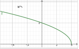
Answer.

horizontal shift of square root $y = \sqrt{x}$
🔗

🔗
vertical shift of cube root $y = \sqrt[3]{x}$
🔗

🔗
vertical shift of absolute value $y = | x |$
🔗

🔗
vertical flip of reciprocal $y = \frac{1}{x}$
🔗

🔗
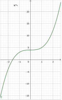
vertical flip and vertical shift of cube $y = x^{3}$
🔗

🔗
vertical flip and vertical shift of inverse-square $y = \frac{1}{x^{2}}$
🔗

🔗

🔗

5.3.4.31.

Answer.

$x < 2$

🔗
$x > \frac{- 2}{3}$

🔗

🔗

5.3.4.33.

Answer.

$41$
🔗

🔗
no solution

🔗
$29 < x \leq 61$
🔗

🔗

🔗

5.4 Direct Variation
5.4.6 Problem Set 5.4

Warm Up

5.4.6.1.

Answer.

$- 10$

🔗
$- 16, 20$

🔗

🔗

Skills Practice

5.4.6.3.

Answer.

$y = 0.3 x$

🔗
$x$ $2$ $5$ $8$ $12$ $15$

$y$ $- 0.6$ $1.5$ $2.4$ $3.6$ $4.5$

🔗
$y$ doubles also

🔗

🔗

5.4.6.5.

Answer.

(b),

k = 0.5

🔗

5.4.6.7.

Answer.

(c)

🔗

Applications

5.4.6.9.

Answer.

$Price of item$ $18$ $28$ $12$

$Tax$ $1.17$ $1.82$ $0.78$

$Tax / Price$ $0.065$ $0.065$ $0.065$

Yes; $6.5 %$
🔗

🔗
$T = 0.065 p$
🔗

🔗
🔗

🔗

5.4.6.11.

Answer.

$m = 0.165 w$
🔗

$w$ $50$ $100$ $200$ $400$

$m$ $8.25$ $16.5$ $33$ $66$

🔗
19.8 lb
🔗

🔗
303.03 lb
🔗

🔗
It will double.
🔗

🔗

🔗

5.4.6.13.

Answer.

$v = 15.306 d$

🔗
3985 million light-years

🔗
18,979 km/sec

🔗

🔗

5.4.6.15.

Answer.

$P = \frac{1825}{8192} w^{3} \approx 0.228 w^{3}$
🔗

$w$ $10$ $20$ $40$ $80$

$P$ $223$ $1782$ $14, 259$ $114, 074$

🔗
752 kilowatts
🔗

🔗
33.54 mph
🔗

🔗
It is multiplied by 8.
🔗

🔗

🔗

5.4.6.17.

Answer.

$d = 0.005 v^{2}$
🔗

🔗
50 m
🔗

🔗

🔗

5.4.6.19.

Answer.

$W = 600 d^{2}$
🔗

🔗
864 newtons
🔗

🔗

🔗

5.4.6.20.

Answer.

Wind resistance quadruples.
🔗

🔗
It is one-ninth as great.
🔗

🔗
It is decreased by 19% because it is 81% of the original.
🔗

🔗

🔗

5.5 Inverse Variation
5.5.4 Problem Set 5.5

Warm Up

5.5.4.1.

Answer.

R = \frac{1}{3} I .

Not inverse variation.

🔗

5.5.4.3.

Answer.

W = 32, 000 - d

Not inverse variation.

🔗

Skills Practice

5.5.4.5.

Answer.

(c)

🔗

5.5.4.7.

Answer.

$y = \frac{120}{x}$

🔗
$x$ $4$ $8$ $20$ $30$ $40$

$y$ $30$ $15$ $6$ $4$ $3$

🔗
$y$ is divided by 2

🔗

🔗

5.5.4.9.

Answer.

(b),

k = 72

🔗

5.5.4.11.

Answer.

(c)

🔗

Applications

5.5.4.13.

Answer.

$Width (feet)$ $2$ $2.5$ $3$

$Length (feet)$ $12$ $9.6$ $8$

$Length \times width$ $24$ $24$ $24$

$24$ square feet
🔗

🔗
$L = \frac{24}{w}$
🔗

🔗
🔗

🔗

5.5.4.15.

Answer.

$B = \frac{88}{d}$
🔗

$d$ $1$ $2$ $12$ $24$

$B$ $88$ $44$ $7.3$ $3.7$

🔗
$8.8$ milligauss
🔗

🔗
More than $20.47$ in
🔗

🔗
It is one half as strong.
🔗

🔗

🔗

5.5.4.17.

Answer.

645

🔗
$D = \frac{64, 500}{n}$

🔗
215

🔗

🔗

5.5.4.18.

Answer.

$m = \frac{8}{p}$
🔗

🔗
0.8 ton
🔗

🔗

🔗

5.5.4.20.

Answer.

$T = \frac{4000}{d}$
🔗

🔗
$8^{\circ}$ C
🔗

🔗

🔗

5.5.4.22.

Answer.

It is one-fourth the original illumination.
🔗

🔗
It is one-ninth the illumination.
🔗

🔗
It is 64% of the illumination.
🔗

🔗

🔗

5.6 Functions as Models
5.6.6 Problem Set 5.6

Warm Up

5.6.6.1.

Answer.

$(0, \infty)$

🔗
none

🔗
$(- i n f t y, 0)$

🔗
none

🔗

🔗

5.6.6.3.

Answer.

none

🔗
$(0, \infty)$

🔗
none

🔗
none

🔗

🔗

5.6.6.5.

Answer.

$(- i n f t y, 0)$

🔗
none

🔗
$(0, \infty)$

🔗
none

🔗

🔗

5.6.6.7.

Answer.

$s = h (t)$

🔗
After 3 seconds, the duck is at a height of 7 meters.

🔗

🔗

Skills Practice

5.6.6.9.

Answer.

Increasing
🔗

🔗
Concave up
🔗

🔗

🔗

5.6.6.11.

Answer.

y = \frac{k}{x}

🔗

Applications

5.6.6.13.

Answer.

(b)

🔗

5.6.6.15.

Answer.

(a)

🔗

5.6.6.17.

Answer.

(b)

🔗

5.6.6.19.

Answer.

II
🔗

🔗
IV
🔗

🔗
I
🔗

🔗
III
🔗

🔗

🔗

5.6.6.21.

Answer.

y = x^{3}

stretched or compressed vertically

🔗

🔗

5.6.6.23.

Answer.

y = \frac{1}{x}

stretched or compressed vertically

🔗

🔗

5.6.6.25.

Answer.

y = \sqrt{x}

🔗

🔗

5.6.6.27.

Answer.

Table (4), Graph (C)
🔗

🔗
Table (3), Graph (B)
🔗

🔗
Table (1), Graph (D)
🔗

🔗
Table (2), Graph (A)
🔗

🔗

🔗

5.6.6.29.

Answer.

III
🔗

🔗
3
🔗

🔗

🔗

Absolute Value

5.6.6.1.

Answer.

$| x | = 6$
🔗

🔗
🔗

🔗

5.6.6.3.

Answer.

$| p + 3 | = 5$
🔗

🔗
🔗

🔗

5.6.6.5.

Answer.

$| t - 6 | < 3$
🔗

🔗
🔗

🔗

5.6.6.7.

Answer.

$| b + 1 | \geq 0.5$
🔗

🔗
🔗

🔗

5.6.6.9.

Answer.

$x = - 5$ or $x = - 1$
🔗

🔗
$- 7 \leq x \leq 1$
🔗

🔗
$x < - 8$ or $x > 2$
🔗

🔗

🔗

5.6.6.11.

Answer.

$x = 4$
🔗

🔗
No solution
🔗

🔗
No solution
🔗

🔗

🔗

5.6.6.13.

Answer.

x = \frac{- 3}{2}

x = \frac{5}{2}

🔗

5.6.6.15.

Answer.

q = \frac{- 7}{3}

🔗

5.6.6.17.

Answer.

b = - 14

b = 10

🔗

5.6.6.19.

Answer.

w = \frac{13}{2}

w = \frac{15}{2}

🔗

5.6.6.21.

Answer.

No solution

🔗

5.6.6.23.

Answer.

No solution

🔗

5.6.6.25.

Answer.

\frac{- 9}{2} < x < \frac{- 3}{2}

🔗

5.6.6.27.

Answer.

d \leq - 2

d \geq 5

🔗

5.6.6.29.

Answer.

All real numbers

🔗

5.6.6.31.

Answer.

1.4 < t < 1.6

🔗

5.6.6.33.

Answer.

T \leq 3.2

T \geq 3.3

🔗

5.6.6.35.

Answer.

No solution

🔗

5.7 Chapter 5 Summary and Review
5.7.3 Chapter 5 Review Problems

5.7.3.1.

Answer.

A function: Each

x

has exactly one associated

y

-value.

🔗

5.7.3.2.

Answer.

Not a function

🔗

5.7.3.3.

Answer.

Not a function: The IQ of

98

has two possible SAT scores.

🔗

5.7.3.4.

Answer.

A function

🔗

5.7.3.5.

Answer.

N (10) = 7000 :

Ten days after the new well is opened, the company has pumped a total of

7000

barrels of oil.

🔗

5.7.3.6.

Answer.

H (16) = 3 :

At 16 mph, the trip takes 3 hours.

🔗

5.7.3.7.

Answer.

F (0) = 1, F (- 3) = \sqrt{37}

🔗

5.7.3.8.

Answer.

G (0) = - 2, G (20) = \sqrt[3]{12}

🔗

5.7.3.9.

Answer.

h (8) = - 6, h (- 8) = - 14

🔗

5.7.3.10.

Answer.

m (5) = 6, m (- 40) = - 4.8

🔗

5.7.3.11.

Answer.

$P (0) = 5$

🔗
x=5,~x=1

🔗

🔗

5.7.3.12.

Answer.

R(0)=2

🔗
$x = 2, x = - 2$

🔗

🔗

5.7.3.13.

Answer.

$f (- 2) = 3, f (2) = 5$
🔗

🔗
$t = 1, t = 3$
🔗

🔗
$t$ -intercepts $(- 3, 0), (4, 0);$ $f (t)$ -intercept: $(0, 2)$
🔗

🔗
Maximum value of $5$ occurs at $t = 2$
🔗

🔗

🔗

5.7.3.14.

Answer.

$P (- 3) = - 2, P (3) = 3$
🔗

🔗
$z = - 5, \frac{- 1}{2}, 4$
🔗

🔗
$(- 4, 0), (- 1, 0), (5, 0);$ $(0, 3)$
🔗

🔗
Maximum value of $- 3$ occurs at $z = - 2$
🔗

🔗

🔗

5.7.3.15.

Answer.

Function

🔗

5.7.3.16.

Answer.

not a function

🔗

5.7.3.17.

Answer.

Not a function

🔗

5.7.3.18.

Answer.

Function

🔗

5.7.3.19.

Answer.

$line$

🔗

5.7.3.21.

Answer.

$line$

🔗

5.7.3.23.

Answer.

$x = \frac{1}{2} = 0.5$
🔗

🔗
$x = \frac{27}{8} \approx 3.4$
🔗

🔗
$x > 4.9$
🔗

🔗
$x \leq 2.0$
🔗

🔗

🔗

5.7.3.24.

Answer.

$x = 0.4$
🔗

🔗
$x = 3.2$
🔗

🔗
$0 < x \leq 4.5$
🔗

🔗
$x < 0$ or $x > 0.2$
🔗

🔗

🔗

5.7.3.25.

Answer.

$x \approx \pm 5.8$
🔗

🔗
$x = \pm 0.4$
🔗

🔗
$- 2.5 < x < 0$ or $0 < x < 2.5$
🔗

🔗
$x \leq - 0.5$ or $x \geq 0.5$
🔗

🔗

🔗

5.7.3.26.

Answer.

$x = 0.5$
🔗

🔗
$x = 2.9$
🔗

🔗
$0 \leq x < 2.3$
🔗

🔗
$x \geq 1.7$
🔗

🔗

🔗

5.7.3.27.

Answer.

y = 1.2 x^{2}

🔗

5.7.3.28.

Answer.

y = 54 x

🔗

5.7.3.29.

Answer.

y = \frac{20}{x}

🔗

5.7.3.30.

Answer.

y = \frac{720}{x^{2}}

🔗

5.7.3.31.

Answer.

$d = 1.75 t^{2}$
🔗

🔗
63 cm
🔗

🔗

🔗

5.7.3.32.

Answer.

$V = \frac{4 T}{P}$
🔗

🔗
$32$
🔗

🔗

🔗

5.7.3.33.

Answer.

480

bottles

🔗

5.7.3.34.

Answer.

14.0625 lumens

🔗

5.7.3.35.

Answer.

$w = \frac{k}{r^{2}}$
🔗

🔗
🔗
$3960 \sqrt{3} \approx 6860$ miles
🔗

🔗

🔗

5.7.3.37.

Answer.

🔗

5.7.3.38.

Answer.

$oven temprature$

🔗

5.7.3.39.

Answer.

🔗

5.7.3.41.

Answer.

🔗

5.7.3.43.

Answer.

🔗
$g (x) = \frac{24}{x}$
🔗

🔗

🔗

5.7.3.44.

Answer.

$decreasing cubic$

🔗
$F (x) = - x^{3}$
🔗

🔗

🔗

5.7.3.45.

Answer.

$x$ $0$ $4$ $8$ $14$ $16$ $22$

$y$ $24$ $20$ $16$ $10$ $8$ $2$

🔗
$y = 24 - x$
🔗

🔗

🔗

5.7.3.46.

Answer.

$x$ $0$ $4$ $10$ $12$ $14$ $16$

$y$ $0$ $6$ $15$ $18$ $21$ $24$

🔗
$y = \frac{3}{2} x$
🔗

🔗

🔗

5.7.3.47.

Answer.

$x$ $0$ $1$ $4$ $9$ $16$ $25$

$y$ $0$ $1$ $2$ $3$ $4$ $5$

🔗
$y = \sqrt{x}$
🔗

🔗

🔗

5.7.3.48.

Answer.

$x$ $0.25$ $0.50$ $1.00$ $1.50$ $2.00$ $4.00$

$y$ $4.00$ $2.00$ $1.00$ $0.67$ $0.50$ $0.25$

🔗
$y = \frac{1}{x}$
🔗

🔗

🔗

5.7.3.49.

Answer.

$x$ $- 3$ $- 2$ $- 1$ $0$ $1$ $2$

$y$ $5$ $0$ $- 3$ $- 4$ $- 3$ $0$

🔗
$y = x^{2} - 4$
🔗

🔗

🔗

5.7.3.50.

Answer.

$x$ $- 3$ $- 2$ $- 1$ $0$ $1$ $4$

$y$ $0$ $5$ $8$ $9$ $8$ $- 7$

🔗
$y = 9 - x^{2}$
🔗

🔗

🔗

6 Powers and Roots
6.1 Integer Exponents
6.1.5 Problem Set 6.1

Warm Up

6.1.5.1.

Answer.

$- 2 z^{2}$

🔗
$- 24 z^{4}$

🔗

🔗

6.1.5.3.

Answer.

$- 12 x^{3} y^{4}$

🔗
$\frac{1}{4 a b^{4}}$

🔗

🔗

6.1.5.5.

Answer.

$4 x^{10} y^{14}$

🔗
$x^{4} y$

🔗

🔗

Skills Practice

6.1.5.7.

Answer.

$9$

🔗
$\frac{1}{9}$

🔗
$9$

🔗
$\frac{1}{9}$

🔗
$- 9$

🔗
$\frac{- 1}{9}$

🔗

🔗

6.1.5.9.

Answer.

$40$

🔗
$\frac{5}{8}$

🔗
$\frac{5}{8}$

🔗
$\frac{1}{40}$

🔗
$40$

🔗
$\frac{8}{5}$

🔗

🔗

6.1.5.11.

Answer.

$\frac{3}{4}$

🔗
$\frac{1}{8}$

🔗
$\frac{1}{2}$

🔗
$\frac{9}{4}$

🔗
$\frac{1}{6}$

🔗
$2$

🔗
$\frac{4}{3}$

🔗
$8$

🔗

🔗

6.1.5.13.

Answer.

$\frac{1}{(m - n)^{2}}$

🔗
$\frac{1}{y^{2}} + \frac{1}{y^{3}}$

🔗
$\frac{2 p}{q^{4}}$

🔗
$\frac{- 5 x^{5}}{y^{2}}$

🔗

🔗

6.1.5.15.

Answer.

1.25

🔗

6.1.5.17.

Answer.

0.2

🔗

6.1.5.19.

Answer.

$\frac{20}{x^{3}}$

🔗
$\frac{1}{3 u^{12}}$

🔗
$5^{8} t$

🔗

🔗

6.1.5.21.

Answer.

$\frac{1}{3} x + 3 x^{- 1}$

🔗
$\frac{1}{4} x^{- 2} - \frac{3}{2} x^{- 1}$

🔗

🔗

6.1.5.23.

Answer.

x - 3 + 2 x^{- 1}

🔗

6.1.5.25.

Answer.

- 4 - 2 u^{- 1} + 6 u^{- 2}

🔗

6.1.5.27.

Answer.

4 x^{- 2} (x^{4} + 4)

🔗

6.1.5.29.

Answer.

$2.85 \times 10^{2}$

🔗
$8.372 \times 10^{6}$

🔗
$2.4 \times 10^{- 2}$

🔗
$5.23 \times 10^{- 4}$

🔗

🔗

Applications

6.1.5.31.

Answer.

$x$ $1$ $2$ $4.5$ $6.2$ $9.3$

$g (x)$ $1$ $0.125$ $0.011$ $0.0042$ $0.0012$

🔗
they decrease
🔗

🔗
$x$ $1.5$ $0.6$ $0.1$ $0.03$ $0.002$

$f (x)$ $0.30$ $4.63$ $1000$ $37, 037$ $125 \times 10^{6}$

🔗
they increase
🔗

🔗

🔗

6.1.5.33.

Answer.

$P = 0.355 v^{3}$

🔗
$v \approx 52.03$ mph
🔗

🔗
3.375

🔗

🔗

6.1.5.35.

Answer.

$d = 50 f^{- 1}$

🔗
The are of the aperture decreases by a factor of 0.5 at each $f$ -stop.

🔗

🔗

6.1.5.36.

Answer.

$1.905 \times 10^{13}$

🔗
$57,552.87

🔗

🔗

6.2 Roots and Radicals
6.2.9 Problem Set 6.2

Warm Up

6.2.9.1.

Answer.

13; 4; 3; 10; 6; 7

🔗

6.2.9.3.

Answer.

$1.414$

🔗
$4.217$

🔗
$1.125$

🔗
$0.140$

🔗
$2.782$

🔗
$3.162$

🔗

🔗

Skills Practice

6.2.9.5.

Answer.

$- 3$

🔗
$u n d e f i n e d$

🔗
$- 3$

🔗
$- 3$

🔗

🔗

6.2.9.7.

Answer.

$\sqrt{7}$
🔗

🔗
$3 \sqrt[4]{x}$
🔗

🔗
$\sqrt[4]{3 x}$
🔗

🔗

🔗

6.2.9.9.

Answer.

$5^{1 / 2}$
🔗

🔗
$(4 y)^{1 / 3}$
🔗

🔗
$5 x^{1 / 3}$
🔗

🔗

🔗

6.2.9.11.

Answer.

\frac{1}{4} x^{1 / 2} - 2 x^{- 1 / 2} + \frac{1}{\sqrt{2}} x

🔗

6.2.9.13.

Answer.

x^{0.5} + x^{- 0.25} - 1

🔗

6.2.9.15.

Answer.

x = 91.125

🔗

6.2.9.17.

Answer.

x = \frac{19}{2}

🔗

6.2.9.19.

Answer.

x = \pm \sqrt{30}

🔗

6.2.9.21.

Answer.

L = \frac{g T^{2}}{4 π^{2}}

🔗

6.2.9.23.

Answer.

M = \frac{d^{3} m}{16 r^{2}}

🔗

6.2.9.25.

Answer.

A = \frac{E}{S T^{4}}

🔗

6.2.9.27.

Answer.

I

🔗
III

🔗
II

🔗
III

🔗

🔗

6.2.9.29.

Answer.

$G (x) = 3.7 x^{1 / 3}$
🔗

🔗
$H (x) = 85^{1 / 4} x^{1 / 4}$
🔗

🔗
$F (t) = 25 t^{- 1 / 5}$
🔗

🔗

🔗

Applications

6.2.9.31.

Answer.

$L$ (feet) $200$ $400$ $600$ $800$ $1000$

$v_{max}$ (knots) $18.4$ $26$ $31.8$ $36.8$ $41.1$

🔗
$maximum velocity$

🔗
50.4 knots

🔗
$maximum and cruise velocities$

🔗
31 knots, 62%

🔗

🔗

6.2.9.33.

Answer.

$T = \frac{2 π}{\sqrt{32}} L^{1 / 2}$
🔗

🔗
$10.54$ sec
🔗

🔗
🔗

🔗

6.2.9.35.

Answer.

$87.68; $72.00
🔗

🔗
1989; 2013
🔗

🔗

🔗

6.2.9.36.

Answer.

$6.5 \times 10^{- 13}$ cm; $1.17 \times 10^{- 36} {cm}^{3}$
🔗

🔗
$1.8 \times 10^{14} g / {cm}^{3}$
🔗

🔗
Element Carbon Potassium Cobalt Technetium Radium

Mass
number, $A$ $14$ $40$ $60$ $99$ $226$

Radius, $r$
( $10^{- 13}$ cm) $3.1$ $4.4$ $5.1$ $6$ $7.9$

🔗
🔗

🔗

6.2.9.37.

Answer.

132.6 km

🔗

6.2.9.39.

Answer.

🔗
$x = 36$
🔗

🔗

🔗

6.3 Rational Exponents
6.3.7 Problem Set 6.3

Warm Up

6.3.7.1.

Answer.

4; 4

🔗
15.59; 15.59

🔗
$8; - 81$

🔗

🔗

6.3.7.3.

Answer.

$2 y^{3}$
🔗

🔗
$3 x^{2}$
🔗

🔗
$2 x^{2} y^{9}$
🔗

🔗
$- 3 a^{2} b^{3}$
🔗

🔗
$4 x^{2} y^{6}$
🔗

🔗
$- 2 x^{5} y$
🔗

🔗

🔗

Skills Practice

6.3.7.5.

Answer.

$\sqrt[4]{y^{3}}$
🔗

🔗
$\frac{1}{\sqrt[7]{a^{2}}}$
🔗

🔗
$\frac{1}{\sqrt[5]{s^{3} t^{3}}}$
🔗

🔗

🔗

6.3.7.7.

Answer.

$y^{3 / 2}$
🔗

🔗
$6 a^{3 / 5} b^{3 / 5}$
🔗

🔗
$- 2 n q^{- 11 / 8}$
🔗

🔗

🔗

6.3.7.9.

Answer.

4 a^{2}

🔗

6.3.7.11.

Answer.

4 w^{3 / 2}

🔗

6.3.7.13.

Answer.

\frac{1}{2 k^{1 / 4}}

🔗

6.3.7.15.

Answer.

x = 64

🔗

6.3.7.17.

Answer.

x = 1.157

🔗

6.3.7.19.

Answer.

29.524

🔗

6.3.7.21.

Answer.

\frac{13}{3}

🔗

6.3.7.23.

Answer.

2 x - x^{2 / 3}

🔗

6.3.7.25.

Answer.

2 x^{1 / 2} - x^{1 / 4} - 1

🔗

6.3.7.27.

Answer.

x (x^{1 / 2} + 1)

🔗

6.3.7.29.

Answer.

\frac{a^{2 / 3} + a^{1 / 3} - 1}{a^{1 / 3}}

🔗

6.3.7.31.

Answer.

$x$	$0$	$1$	$2$	$3$	$4$	$5$	$6$
$f (x)$	$0$	$1$	$2.5$	$4.3$	$6.4$	$8.5$	$10.9$
$g (x)$	$0$	$1$	$2.8$	$5.2$	$8$	$11.2$	$14.7$

$power functions$

🔗

6.3.7.33.

Answer.

$2.83$
🔗

🔗
$3.30$
🔗

🔗

🔗

Applications

6.3.7.35.

Answer.

$t$ $5$ $10$ $15$ $20$

$I (t)$ $131$ $199$ $254$ $302$

🔗
20 days

🔗
🔗

🔗

6.3.7.37.

Answer.

$A$ $10$ $100$ $1000$ $5000$ $10, 000$

$S$ $25$ $42$ $69$ $98$ $115$

🔗
🔗
81, 71
🔗

🔗
126,000 sq km
🔗

🔗

🔗

6.3.7.39.

Answer.

1.62

🔗
1.62

🔗
0.84; 0.84

🔗

🔗

6.3.7.41.

Answer.

15 days, 28 days

🔗
$\frac{I (m) \times W (m)}{m} = 0.18 m^{- 0.041}$

🔗
$m^{- 0.041}$ is close to 1

🔗

🔗

6.3.7.43.

Answer.

$p = K^{1 / 2} a^{3 / 2}$

🔗
1.88 years

🔗

🔗

6.4 Working with Radicals
6.4.6 Problem Set 6.4

Warm Up

6.4.6.1.

Answer.

🔗

6.4.6.3.

Answer.

Yes

🔗

6.4.6.5.

Answer.

\sqrt{a b} = \sqrt{a} \sqrt{b}

\sqrt{\frac{a}{b}} = \frac{\sqrt{a}}{\sqrt{b}}

🔗

Skills Practice

6.4.6.7.

Answer.

$3 \sqrt{2}$
🔗

🔗
$2 \sqrt[3]{3}$
🔗

🔗
$- 2 \sqrt[4]{4} = - 2 \sqrt{2}$
🔗

🔗

🔗

6.4.6.9.

Answer.

$x^{3} \sqrt[3]{x}$
🔗

🔗
$3 z \sqrt{3 z}$
🔗

🔗
$2 a^{2} \sqrt[4]{3 a}$
🔗

🔗

🔗

6.4.6.11.

Answer.

$2 \sqrt{4 - x^{2}}$
🔗

🔗
$A \sqrt[3]{8 + A^{3}}$
🔗

🔗

🔗

6.4.6.13.

Answer.

$\sqrt[3]{a b^{2}}$
🔗

🔗
$x \sqrt{x y}$
🔗

🔗

🔗

6.4.6.15.

Answer.

$4 \sqrt[3]{3}$

🔗
$- \sqrt[3]{2}$

🔗

🔗

6.4.6.17.

Answer.

$6 \sqrt{3} + 6 \sqrt{5}$

🔗
$3 k \sqrt{3} - 3 k^{2} \sqrt{2}$

🔗

🔗

6.4.6.19.

Answer.

$x - 9$

🔗
$- 4 + \sqrt{6}$

🔗

🔗

6.4.6.21.

Answer.

$3 - \sqrt{5}$

🔗
$\frac{- 4 + \sqrt{2}}{2}$

🔗
$\frac{2 a - \sqrt{2}}{2 a}$

🔗

🔗

6.4.6.23.

Answer.

$\frac{\sqrt{14 x}}{6}$

🔗
$\frac{\sqrt{2 a b}}{b}$

🔗

🔗

6.4.6.25.

Answer.

$- 2 1 - \sqrt{3}$

🔗
$\frac{x (x + \sqrt{3}}{x^{2} - 3}$

🔗

🔗

Applications

6.4.6.27.

Answer.

x^{2} + 4 x = (4 - 4 \sqrt{5} + 5) + (8 + 4 \sqrt{5}) = 1

🔗

6.4.6.29.

Answer.

$\frac{w \sqrt{3}}{2}$

🔗
$\frac{w^{2} \sqrt{3}}{4}$

🔗

🔗

6.5 Radical Equations
6.5.6 Problem Set 6.5

Warm Up

6.5.6.1.

Answer.

$z = 4$

🔗
$w = 8$

🔗

🔗

6.5.6.3.

Answer.

$square root graph$

🔗
13

🔗

🔗

6.5.6.5.

Answer.

$x$ $y$

$- 25$ $6.92$

$- 20$ $6.71$

$- 15$ $6.47$

$- 10$ $6.15$

$- 5$ $3.21$

$0$ $4$

$5$ $2.29$

$10$ $1.85$

$15$ $1.53$

$20$ $1.29$

$grid$

🔗
$- 8$

🔗

🔗

Skills Practice

6.5.6.7.

Answer.

\frac{- 1}{3}

🔗

6.5.6.9.

Answer.

5

🔗

6.5.6.11.

Answer.

5

🔗

6.5.6.13.

Answer.

🔗

6.5.6.15.

Answer.

🔗

6.5.6.17.

Answer.

$2 | x |$

🔗
$| x - 5 |$

🔗
$| x - 3 |$

🔗

🔗

Applications

6.5.6.19.

Answer.

1.25 mi; 6600 ft

🔗
$h = (\frac{d}{89.4})^{2}$

🔗

🔗

6.5.6.21.

Answer.

339.39 cubic in

🔗
$V = 12.57 r^{3}$

🔗

🔗

6.5.6.23.

Answer.

b = \pm \sqrt{a^{2} - c^{2}}

🔗

6.5.6.25.

Answer.

W = \frac{v}{1 - (\frac{D}{S})^{3}}

🔗

6.6 Chapter 6 Summary and Review
6.6.3 Chapter 6 Review Problems

6.6.3.1.

Answer.

$\frac{1}{81}$

🔗
$\frac{1}{64}$

🔗

🔗

6.6.3.2.

Answer.

$9$

🔗
$75$

🔗

🔗

6.6.3.3.

Answer.

$\frac{1}{243 m^{5}}$

🔗
$\frac{- 7}{y^{8}}$

🔗

🔗

6.6.3.4.

Answer.

$\frac{1}{a} + \frac{1}{a^{2}}$

🔗
$\frac{3 r^{2}}{q^{9}}$

🔗

🔗

6.6.3.5.

Answer.

$\frac{2}{c^{3}}$

🔗
$\frac{99}{z^{2}}$

🔗

🔗

6.6.3.6.

Answer.

$\frac{d^{8}}{16 k^{12}}$

🔗
$\frac{2}{5} w^{14}$

🔗

🔗

6.6.3.7.

Answer.

$1.018 \times 10 - 9$ sec, or 0.000 000 001 018 sec

🔗
8 min 20 sec

🔗

🔗

6.6.3.8.

Answer.

1,200,000,000,000 hr, or 78,904,109,590 yr

🔗

6.6.3.9.

Answer.

5000 sec, or 83 min

🔗
$\frac{1}{10}$

🔗
42 yr

🔗

🔗

6.6.3.10.

Answer.

Planet Density

Mercury 5426

Venus 5244

Earth 5497

Mars 3909

Jupiter 1241

Saturn 620

Uranus 1238

Neptune 1615

Pluto 2355

🔗
Mercury, Venus, Earth, and Mars

🔗

🔗

6.6.3.11.

Answer.

$25 \sqrt{m}$
🔗

🔗
$\frac{8}{\sqrt[3]{n}}$
🔗

🔗

🔗

6.6.3.12.

Answer.

$\sqrt[3]{(13 d)^{3}}$
🔗

🔗
$6 \sqrt[5]{x^{2} y^{3}}$
🔗

🔗

🔗

6.6.3.13.

Answer.

$\frac{1}{\sqrt[4]{27 q^{3}}}$
🔗

🔗
$7 \sqrt{u^{3} v^{3}}$
🔗

🔗

🔗

6.6.3.14.

Answer.

$\sqrt{a^{2} + b^{2}}$
🔗

🔗
$\sqrt[4]{16 - x^{2}}$
🔗

🔗

🔗

6.6.3.15.

Answer.

$2 x^{2 / 3}$
🔗

🔗
$\frac{1}{4} x^{1 / 4}$
🔗

🔗

🔗

6.6.3.16.

Answer.

$z^{5 / 2}$
🔗

🔗
$z^{4 / 3}$
🔗

🔗

🔗

6.6.3.17.

Answer.

$6 b^{- 3 / 4}$
🔗

🔗
$\frac{- 1}{3} b^{- 1 / 3}$
🔗

🔗

🔗

6.6.3.18.

Answer.

$- 4 a^{- 1 / 2}$
🔗

🔗
$2 a^{- 3 / 2}$
🔗

🔗

🔗

6.6.3.19.

Answer.

112 kg

🔗

6.6.3.20.

Answer.

Height: 2.673 in; diameter: 5.346 in

🔗

6.6.3.21.

Answer.

480
🔗

🔗
498
🔗

🔗

🔗

6.6.3.22.

Answer.

294 sq in
🔗

🔗
90 lb
🔗

🔗

🔗

6.6.3.23.

Answer.

🔗
283
🔗

🔗
2051
🔗

🔗

🔗

6.6.3.25.

Answer.

$power function$

🔗
$7114.32
🔗

🔗

🔗

6.6.3.27.

Answer.

It is the cost of producing the first ship.
🔗

🔗
$C = \frac{12}{\sqrt[8]{x}}$ million
🔗

🔗
About $11 million; about 8.3% ; about 8.3%>
🔗

🔗
About 8.3%
🔗

🔗

🔗

6.6.3.29.

Answer.

$4096$

🔗
$\frac{1}{8}$

🔗
$36 \sqrt{3} \approx 62.35$

🔗
$400, 000$

🔗

🔗

6.6.3.30.

Answer.

$- 27$

🔗
$\frac{- 3}{4}$

🔗
$- 3 \sqrt[3]{400} \approx - 22.1$

🔗
$- 300$

🔗

🔗

6.6.3.31.

Answer.

169

🔗

6.6.3.32.

Answer.

49

🔗

6.6.3.33.

Answer.

16

🔗

6.6.3.34.

Answer.

- 16

🔗

6.6.3.35.

Answer.

1, 4

🔗

6.6.3.36.

Answer.

8

🔗

6.6.3.37.

Answer.

9

🔗

6.6.3.38.

Answer.

12

🔗

6.6.3.39.

Answer.

7

🔗

6.6.3.40.

Answer.

\pm 8

🔗

6.6.3.41.

Answer.

5

🔗

6.6.3.42.

Answer.

4

🔗

6.6.3.43.

Answer.

g = \frac{2 v}{t^{2}}

🔗

6.6.3.44.

Answer.

r = \frac{\pm \sqrt{3 q^{2} - 6 q + 7}}{2}

🔗

6.6.3.45.

Answer.

p = \pm 2 \sqrt{R^{2} - R}

🔗

6.6.3.46.

Answer.

r = \pm \sqrt{2 q^{3} - 1}

🔗

6.6.3.47.

Answer.

$\frac{5 p^{4}}{a^{2}} \sqrt{5 p}$

🔗
$\frac{2}{w^{2}} \sqrt[3]{3 v^{2}}$

🔗

🔗

6.6.3.48.

Answer.

$a^{2} b$

🔗
$x y$

🔗

🔗

6.6.3.49.

Answer.

$2 \sqrt[3]{a^{3} - 2 b^{6}}$

🔗
$- 4 a b^{2} \sqrt[3]{2}$

🔗

🔗

6.6.3.50.

Answer.

$2 t \sqrt{1 + 6 t^{4}}$

🔗
$4 t^{4} \sqrt{6}$
🔗

🔗

🔗

6.6.3.51.

Answer.

$x^{2} - 4 x \sqrt{x} + 4 x$

🔗
$x^{2} - 4 x$

🔗

🔗

6.6.3.52.

Answer.

$14 - 4 \sqrt{6}$

🔗
$2 a - 4 b$

🔗

🔗

6.6.3.53.

Answer.

$\frac{7 \sqrt{5 y}}{5 y}$

🔗
$3 \sqrt{2 d}$

🔗

🔗

6.6.3.54.

Answer.

$\frac{\sqrt{33 r s}}{11 s}$

🔗
$\frac{\sqrt{13 m}}{m}$

🔗

🔗

6.6.3.55.

Answer.

$\frac{- 3 \sqrt{a} + 6}{a - 4}$

🔗
$\frac{- 3 \sqrt{z} - 12}{z - 16}$

🔗

🔗

6.6.3.56.

Answer.

$\frac{2 x^{2} + x \sqrt{3} - 3}{x^{2} - 3}$

🔗
$\frac{5 m^{2} - 7 m \sqrt{3} + 6}{25 m^{2} - 12}$

🔗

🔗

7 Exponential Functions
7.1 Exponential Growth and Decay
7.1.7 Problem Set 7.1

Warm Up

7.1.7.1.

Answer.

$28

🔗
#31.36

🔗
No. It increase by 12% of different amounts.

🔗

🔗

7.1.7.3.

Answer.

Decreased by 1%.

🔗

7.1.7.5.

Answer.

🔗

7.1.7.7.

Answer.

\pm 1.2

🔗

7.1.7.9.

Answer.

- 2.14;

0.14

🔗

Skills Practice

7.1.7.11.

Answer.

$P = 1200 + 150 t;$ 1650
🔗

🔗
$P = 1200 \cdot {1.5}^{t};$ 4050
🔗

🔗

🔗

7.1.7.13.

Answer.

$V = 18, 000 - 2000 t;$ $8000
🔗

🔗
$V = 18, 000 \cdot {0.8}^{t};$ $5898.24
🔗

🔗

🔗

7.1.7.15.

Answer.

20%, 2%, 7.5%, 100%, 115%

🔗

7.1.7.17.

Answer.

$P_{0} = 4, b = 2^{1 / 3}$
🔗

🔗
$P (t) = 4 \cdot 2^{t / 3}$
🔗

🔗

🔗

7.1.7.18.

Answer.

Initial value $80,$ decay factor $\frac{1}{2}$
🔗

🔗
$f (x) = 80 \cdot {(\frac{1}{2})}^{x}$
🔗

🔗

🔗

7.1.7.19.

Answer.

The growth factor is

1.2 .

🔗

$x$	$0$	$1$	$2$	$3$	$4$
$Q$	$20$	$24$	$28.8$	$34.56$	$41.47$

🔗

7.1.7.20.

Answer.

The decay factor is

0.8 .

🔗

$w$	$0$	$1$	$2$	$3$	$4$
$N$	$120$	$96$	$76.8$	$61.44$	$49.15$

🔗

7.1.7.21.

Answer.

The decay factor is

0.8 .

🔗

$t$	$0$	$1$	$2$	$3$	$4$
$C$	$10$	$8$	$6.4$	$5.12$	$4.10$

🔗

7.1.7.22.

Answer.

The growth factor is

1.1 .

🔗

$n$	$0$	$1$	$2$	$3$	$4$
$B$	$200$	$220$	$242$	$266.2$	$292.82$

🔗

Applications

7.1.7.23.

Answer.

Years after 2010 $0$ $1$ $2$ $3$ $4$

Windsurfers $1500$ $1680$ $1882$ $2107$ $2360$

🔗
$S (t) = 1200 (1.12)^{t}$

🔗
$Windsurfer sales exponential growth$

🔗
2644; 5844

🔗

🔗

7.1.7.24.

Answer.

Years after 1983 $0$ $5$ $10$ $15$ $20$

Value of house $20, 000$ $25, 526$ $32, 578$ $41, 579$ $53, 066$

🔗
$V (t) = 200, 000 (1.05)^{t}$

🔗
$house value$

🔗
$359,171.27; $458,403.66

🔗

🔗

7.1.7.25.

Answer.

Weeks $0$ $6$ $12$ $18$ $24$

Bees $2000$ $5000$ $12, 500$ $31, 250$ $78, 125$

🔗
$P (t) = 2000 (2.5)^{t / 6}$

🔗
🔗

🔗

7.1.7.27.

Answer.

Weeks $0$ $2$ $4$ $6$ $8$

Mosquitos $250, 000$ $187, 500$ $140, 625$ $105, 469$ $79, 102$

🔗
$P (t) = 250, 000 (0.75)^{t / 2}$

🔗
🔗
162,280; 68,504

🔗

🔗

7.1.7.29.

Answer.

Years $0$ $3$ $6$ $9$ $12$

Value of boat $15, 000$ $13, 500$ $12, 150$ $10, 935$ $9841.50$

🔗
$V (t) = 15, 000 (0.885)^{t}$

🔗
$motorboat depreciation$

🔗
$4995.52; $4421.04

🔗

🔗

7.1.7.31.

Answer.

$P (t) = 1, 545, 387 b^{t}$

🔗
$b = 1.049; r = 4.9 %$

🔗
3,167,157

🔗

🔗

7.1.7.33.

Answer.

365

🔗
🔗
$N (t) = 365 (0.356)^{t}$

🔗
0.03

🔗

🔗

7.1.7.35.

Answer.

2440 tigers per decade
🔗

🔗
0.765; 23.5%
🔗

🔗
3080; 4656
🔗

🔗

🔗

7.1.7.37.

Answer.

39; 1.045

🔗
36; 1.047

🔗
Species B

🔗

🔗

7.2 Exponential Functions
7.2.6 Problem Set 7.2

Warm Up

7.2.6.1.

Answer.

$3^{x + 4}$
🔗

🔗
$3^{4 x}$
🔗

🔗
$12^{x}$
🔗

🔗

🔗

7.2.6.3.

Answer.

$b^{- 2 t}$
🔗

🔗
$b^{t / 2}$
🔗

🔗
$1$
🔗

🔗

🔗

7.2.6.5.

Answer.

0.06

🔗

Skills Practice

7.2.6.7.

Answer.

\frac{2}{3}

🔗

7.2.6.8.

Answer.

\frac{- 1}{4}

🔗

7.2.6.9.

Answer.

\frac{1}{7}

🔗

7.2.6.11.

Answer.

\frac{- 5}{4}

🔗

7.2.6.13.

Answer.

\pm 2

🔗

7.2.6.15.

Answer.

2.26

🔗

7.2.6.17.

Answer.

$(0, 26);$ increasing
🔗

🔗
$(0, 1.2);$ decreasing
🔗

🔗
$(0, 75);$ decreasing
🔗

🔗
$(0, \frac{2}{3});$ increasing
🔗

🔗

🔗

7.2.6.18.

Answer.

Power
🔗

🔗
Exponential
🔗

🔗
Power
🔗

🔗
Neither
🔗

🔗

🔗

7.2.6.19.

Answer.

$x$	$- 3$	$- 2$	$- 1$	$0$	$1$	$2$	$3$
$f (x) = 3^{x}$	$\frac{1}{27}$	$\frac{1}{9}$	$\frac{1}{3}$	$1$	$3$	$9$	$27$
$g (x) = {(\frac{1}{3})}^{x}$	$27$	$9$	$3$	$1$	$\frac{1}{3}$	$\frac{1}{9}$	$\frac{1}{27}$

🔗

7.2.6.21.

Answer.

Because they are defined by equivalent expressions, (b), (c), and (d) have identical graphs.

🔗

7.2.6.23.

Answer.

0.17; 5.95

🔗

7.2.6.25.

Answer.

$P_{0} = 800$

🔗
$x$ $0$ $1$ $2$

$g (x)$ $800$ $200$ $50$

🔗
$a = \frac{1}{4}$

🔗
$g (x) = 800 (\frac{1}{4})^{x}$

🔗

🔗

7.2.6.27.

Answer.

Power $y = 100 x^{- 1}$
🔗

🔗
Exponential $P = \frac{1}{4} \cdot 2^{x}$
🔗

🔗

🔗

Applications

7.2.6.28.

Answer.

$V (t) = 20, 000 (0.8)^{t / 3}$
🔗

🔗
🔗
6 years
🔗

🔗

🔗

7.2.6.29.

Answer.

$N (t) = 26 (2)^{t / 6}$
🔗

🔗
🔗
72 days later
🔗

🔗

🔗

7.2.6.30.

Answer.

$F_{0} = 400$
🔗

🔗
$b = 1.06$
🔗

🔗
$F (p) = 440 (1.06)^{p}$
🔗

🔗

🔗

7.2.6.31.

Answer.

$S_{0} = 150$
🔗

🔗
$b \approx 0.55$
🔗

🔗
$S (d) = 150 (0.55)^{d}$
🔗

🔗

🔗

7.2.6.32.

Answer.

$x$	$f (x) = x^{2}$	$g (x) = 2^{x}$
$- 2$	$4$	$\frac{1}{4}$
$- 1$	$1$	$\frac{1}{2}$
$0$	$0$	1
$1$	$1$	$2$
$2$	$4$	$4$
$3$	$9$	$8$
$4$	$16$	$16$
$5$	$25$	$32$

$T h r e e$
🔗

🔗
$x = - 0.77, 2, 4$
🔗

🔗
$(- 0.77, 2) \cup (4, \infty)$
🔗

🔗
$g (x)$
🔗

🔗

🔗

7.3 Logarithms
7.3.7 Problem Set 7.3

Warm Up

7.3.7.1.

Answer.

$P (t) = 300 (1.15)^{t}$
🔗

🔗
$500 = 300 (1.15)^{t}$
🔗

🔗
$t \approx 3.65$
🔗

🔗

🔗

Skills Practice

7.3.7.3.

Answer.

$2$
🔗

🔗
$4$
🔗

🔗

🔗

7.3.7.5.

Answer.

$\frac{1}{2}$
🔗

🔗
$- 1$
🔗

🔗

🔗

7.3.7.7.

Answer.

$- 1$
🔗

🔗
$4$
🔗

🔗

🔗

7.3.7.9.

Answer.

$3 < x < 4$
🔗

🔗
$- 1 < y < 0$
🔗

🔗

🔗

7.3.7.11.

Answer.

- 0.23

🔗

7.3.7.13.

Answer.

0.77

🔗

7.3.7.15.

Answer.

2.53

🔗

7.3.7.17.

Answer.

$\log_{t} (16) = \frac{3}{2}$
🔗

🔗
$\log_{0.8} (M) = 1.2$
🔗

🔗

🔗

7.3.7.19.

Answer.

$16^{w} = 256$

🔗
b^{-2} = 9

🔗

🔗

7.3.7.21.

Answer.

$x = \log_{4} (2.5) \approx 2.7$

🔗
$x = \log_{2} (0.2) \approx - 2.3$

🔗

🔗

7.3.7.23.

Answer.

2.77

🔗

Applications

7.3.7.25.

Answer.

2030

🔗
6.2%

🔗

🔗

7.3.7.27.

Answer.

9.60 in

🔗
3.85 mi

🔗

🔗

7.3.7.29.

Answer.

2,018,436
🔗

🔗
5.17%
🔗

🔗
2008
🔗

🔗

🔗

7.3.7.31.

Answer.

$4$
🔗

🔗
$4$
🔗

🔗
$64$
🔗

🔗
$\sqrt[3]{16} \approx 2.52$
🔗

🔗

🔗

7.4 Properties of Logarithms
7.4.5 Problem Set 7.4

Warm Up

7.4.5.1.

Answer.

$\log_{8} (\frac{1}{2}) = \frac{- 1}{3}$
🔗

🔗
$\log_{5} (46) = x$
🔗

🔗

🔗

7.4.5.3.

Answer.

$10^{8}$
🔗

🔗
$2; 6; 8$ Property (1)
🔗

🔗

🔗

7.4.5.5.

Answer.

$b^{3}$
🔗

🔗
$8; 5; 3$ Property (2)
🔗

🔗

🔗

7.4.5.7.

Answer.

$10^{15}$
🔗

🔗
$15; 3$ Property (3)
🔗

🔗

🔗

7.4.5.9.

Answer.

$5$
🔗

🔗
$6$
🔗

🔗
$5$
🔗

🔗

(a) and (c) are equal.

🔗

7.4.5.11.

Answer.

$\log (24) \approx 1.38$
🔗

🔗
$\log (240) \approx 2.38$
🔗

🔗
$\log (230) \approx 2.36$
🔗

🔗

None are equal.

🔗

Skills Practice

7.4.5.13.

Answer.

$\log_{b} (2) + \log_{b} (x)$
🔗

🔗
$\log_{b} (2) - \log_{b} (x)$
🔗

🔗
$3 \log_{b} (x)$
🔗

🔗
$\frac{2}{3} \log_{b} (x)$
🔗

🔗

🔗

7.4.5.15.

Answer.

$\log_{3} (3) + 4 \log_{3} (x)$

🔗
$(1 / t) \log_{5} (1.1)$

🔗
$Extra \left or missing \right$
🔗

🔗
$\log_{2} (5) + x$
🔗

🔗

🔗

7.4.5.17.

Answer.

$\log_{b} (4)$
🔗

🔗
$\log_{4} (x^{2} y^{3})$
🔗

🔗

🔗

7.4.5.19.

Answer.

$\log (2 x^{5 / 2})$
🔗

🔗
$\log (t - 4)$
🔗

🔗

🔗

7.4.5.21.

Answer.

y = \frac{1}{25}

🔗

7.4.5.23.

Answer.

b = 100

🔗

7.4.5.25.

Answer.

2.81

🔗

7.4.5.27.

Answer.

- 1.61

🔗

7.4.5.29.

Answer.

- 12.49

🔗

7.4.5.31.

Answer.

$1.7918$
🔗

🔗
$- 0.9163$
🔗

🔗

🔗

7.4.5.33.

Answer.

(a) and (d)

🔗

7.4.5.35.

Answer.

(a) and (c)

🔗

Applications

7.4.5.37.

Answer.

$S (t) = S_{0} (1.09)^{t}$
🔗

🔗
$4.7$ hours
🔗

🔗

🔗

7.4.5.39.

Answer.

$C (t) = 0.7 (0.80)^{t}$
🔗

🔗
After 2.5 hours
🔗

🔗
🔗

🔗

7.4.5.41.

Answer.

$S (t) = S_{0} \cdot {0.9527}^{t}$
🔗

🔗
28.61 hours
🔗

🔗

🔗

7.4.5.43.

Answer.

k = \frac{\log (\frac{N}{N_{0}})}{t \log (a)}

🔗

7.4.5.45.

Answer.

t = \frac{1}{k} \log (\frac{A}{A_{0}} + 1)

🔗

7.5 Exponential Models
7.5.5 Problem Set 7.5

Warm Up

7.5.5.1.

Answer.

4.16

🔗

7.5.5.3.

Answer.

🔗

7.5.5.5.

Answer.

y = \frac{- 2}{3} x - 1

🔗

7.5.5.7.

Answer.

y = \frac{- 1}{2} x + 4

🔗

Skills Practice

7.5.5.9.

Answer.

P (x) = 8 (0.5)^{x}

🔗

7.5.5.11.

Answer.

y = 1.5 (3) x / 5

🔗

7.5.5.13.

Answer.

$y = 2.6 - 1.3 x$

🔗
$y = 2.5 (0, 5)^{x}$

🔗
🔗

🔗

Applications

7.5.5.15.

Answer.

P (t) = 2000 (2^{t / 5};

14.9%

🔗

7.5.5.17.

Answer.

D (t) = D_{0} (0, 5^{t / 18};

3.8%

🔗

7.5.5.19.

Answer.

$P = P_{0} (2)^{t / 25}$
🔗

🔗
2.81%
🔗

🔗

🔗

7.5.5.21.

Answer.

$\frac{\log (0.5)}{\log (0.946)} \approx 12.5$ hours
🔗

🔗
25 hours
🔗

🔗
🔗

🔗

7.5.5.23.

Answer.

$D (t) = D_{0} (0.5)^{t / 15}$

🔗
After 89.5 years, or in 2060

🔗

🔗

7.5.5.25.

Answer.

$A = A_{0} {(\frac{1}{2})}^{t / 5730}$
🔗

🔗
About 760 years old
🔗

🔗

🔗

7.5.5.27.

Answer.

12.9%

🔗

7.5.5.29.

Answer.

About 11 years

🔗

7.6 Chapter 7 Summary and Review
7.6.3 Chapter 7 Review Problems

7.6.3.1.

Answer.

$D = 8 (1.5)^{t / 5}$
🔗

🔗
$18;$ $44$
🔗

🔗

🔗

7.6.3.3.

Answer.

$M = 100 (0.85)^{t}$
🔗

🔗
$52.2$ mg; $19.7$ mg
🔗

🔗

🔗

7.6.3.5.

Answer.

🔗

7.6.3.7.

Answer.

🔗

7.6.3.9.

Answer.

\frac{- 4}{3}

🔗

7.6.3.11.

Answer.

- 11

🔗

7.6.3.13.

Answer.

4

🔗

7.6.3.15.

Answer.

- 1

🔗

7.6.3.17.

Answer.

- 3

🔗

7.6.3.19.

Answer.

2^{x - 2} = 3

🔗

7.6.3.20.

Answer.

n^{p - 1} = q

🔗

7.6.3.21.

Answer.

\log_{0.3} (x + 1) = - 2

🔗

7.6.3.23.

Answer.

- 1

🔗

7.6.3.25.

Answer.

4

🔗

7.6.3.27.

Answer.

\frac{\log (5.1)}{1.3} \approx 0.5433

🔗

7.6.3.29.

Answer.

\frac{\log (2.9 / 3)}{- 0.7} \approx 0.21

🔗

7.6.3.31.

Answer.

0.054

🔗

7.6.3.32.

Answer.

2.959

🔗

7.6.3.33.

Answer.

0.195

🔗

7.6.3.34.

Answer.

2.823

🔗

7.6.3.35.

Answer.

\log_{b} (x) + \frac{1}{3} \log_{b} (y) - 2 \log_{b} (z)

🔗

7.6.3.37.

Answer.

\frac{4}{3} \log (x) - \frac{1}{3} \log (y)

🔗

7.6.3.39.

Answer.

Missing \left or extra \right

🔗

7.6.3.41.

Answer.

\log (\frac{1}{8})

🔗

7.6.3.43.

Answer.

\frac{\log (63)}{\log (3)} \approx 3.77

🔗

7.6.3.45.

Answer.

\frac{\log (50)}{- 0.3 \log (6)} \approx - 7.278

🔗

7.6.3.47.

Answer.

\frac{\log (N / N_{0})}{k}

🔗

7.6.3.49.

Answer.

$238$
🔗

🔗
$2010$
🔗

🔗

🔗

7.6.3.51.

Answer.

$C = 90 (1.06)^{t}$
🔗

🔗
$ $94.48$
🔗

🔗
$5$ years
🔗

🔗

🔗

8 Polynomial and Rational Functions
8.1 Polynomial Functions
8.1.10 Problem Set 8.1

Warm Up

8.1.10.1.

Answer.

$a^{2} + 2 a b + b^{2}$

🔗
$a^{2} - 2 a b + b^{2}$

🔗

🔗

8.1.10.3.

Answer.

$(x - 7)^{2}$

🔗
cannot be factored

🔗
$(x + 3)^{2}$

🔗
$(x + 8) (x - 8)$

🔗

🔗

Skills Practice

8.1.10.5.

Answer.

(b) and (c) are not polynomials; they have variables in a denominator.

🔗

8.1.10.7.

Answer.

$- 1.9 x^{3} + x + 6.4$

🔗
$- 2 x^{2} + 6 x y + 2 y^{3}$

🔗

🔗

8.1.10.9.

Answer.

4

🔗
5

🔗
7

🔗

🔗

8.1.10.11.

Answer.

$6 a^{4} - 5 a^{3} - 5 a^{2} + 5 a - 1$
🔗

🔗
$y^{4} + 5 y^{3} - 20 y - 16$
🔗

🔗

🔗

8.1.10.13.

Answer.

$1 + 15 \sqrt{t} + 75 t + 125 t \sqrt{t}$
🔗

🔗
$1 - \frac{9}{a} + \frac{27}{a^{2}} - \frac{27}{a^{3}}$
🔗

🔗

🔗

8.1.10.15.

Answer.

$27 a^{3} - 8 b^{3}$

🔗
$8 a^{3} + 27 b^{3}$

🔗

🔗

8.1.10.17.

Answer.

(a - 2 b) (a^{2} + 2 a b + 4 b^{2})

🔗

8.1.10.19.

Answer.

(3 a + 4 b) (9 a^{2} - 12 a b + 16 b^{2})

🔗

8.1.10.21.

Answer.

(4 t^{3} + w^{2}) (16 t^{6} - 4 t^{3} w^{2} + w^{4})

🔗

Applications

8.1.10.23.

Answer.

length: $w + 3;$ height: $w - 2$

🔗
$w^{3} + w^{2} - 6 w$

🔗
$5 w^{2} + w - 12$

🔗

🔗

8.1.10.25.

Answer.

$\frac{2}{3} π r^{3} + π r^{2} h$
🔗

🔗
$V (r) = \frac{14}{3} π r^{3}$
🔗

🔗

🔗

8.1.10.27.

Answer.

$0, 9$
🔗

🔗
$0 \leq x \leq 9;$ $R \geq 0$ for these values
🔗

🔗
🔗
$\frac{28}{3}$ points
🔗

🔗
$36$ points
🔗

🔗
$3$ ml or $8.2$ ml
🔗

🔗

🔗

8.1.10.29.

Answer.

$20$ cm
🔗

🔗
$100$ cm
🔗

🔗

🔗

8.1.10.31.

Answer.

$6 + x + 5 x^{2}$

🔗
$4 - 7 x^{2} - 8 x^{4}$

🔗

🔗

8.2 Algebraic Fractions
8.2.5 Problem Set 8.2

Warm Up

8.2.5.1.

Answer.

$\frac{- 3}{5},$ $\frac{3}{7}$
🔗

🔗
$3$
🔗

🔗
$- 1$

🔗

🔗

8.2.5.3.

Answer.

$\frac{- 4}{3},$ $\frac{40}{399}$
🔗

🔗
$1, - 1$
🔗

🔗
$0$

🔗

🔗

8.2.5.5.

Answer.

$\frac{5}{x}$
🔗

🔗
$\frac{12 b}{7}$

🔗

🔗

8.2.5.7.

Answer.

$\frac{- 8}{5}$

🔗
$\frac{a}{9}$

🔗

🔗

Skills Practice

8.2.5.9.

Answer.

None are correct

🔗

8.2.5.11.

Answer.

cannot be reduced
🔗

🔗
$1$
🔗

🔗
cannot be reduced
🔗

🔗
cannot be reduced
🔗

🔗

🔗

8.2.5.13.

Answer.

(b)

🔗

8.2.5.15.

Answer.

(a)

🔗

8.2.5.17.

Answer.

\frac{a}{a - 3}

🔗

8.2.5.19.

Answer.

\frac{1}{a + b}

🔗

8.2.5.21.

Answer.

\frac{y + 3 x}{y - 3 x}

🔗

8.2.5.23.

Answer.

y - 2

🔗

8.2.5.25.

Answer.

\frac{- a}{a + 1}

🔗

8.2.5.27.

Answer.

\frac{4 z^{2} + 6 z + 9}{2 z + 3}

🔗

Applications

8.2.5.29.

Answer.

30 min
🔗

🔗
50 min
🔗

🔗
50 min
🔗

🔗
6 mph
🔗

🔗
The time increases. If the current is 10 mph, the team will not be able to row upstream
🔗

🔗

🔗

8.2.5.31.

Answer.

$0 \leq p < 100$
🔗

🔗
$p$ $0$ $25$ $50$ $75$ $90$ $100$

$C$ $0$ $120$ $360$ $1080$ $3240$ $- -$

🔗
$curve$

60%
🔗

🔗
$p < 80 %$
🔗

🔗
$p = 100 :$ The cost of extracting more ore grows without bound as the amount extracted approaches 100%.
🔗

🔗

🔗

8.2.5.33.

Answer.

$\frac{200}{2 x - 1}$ square centimeters
🔗

🔗
8; If $x = 13,$ the area of the cross-section is 8 ${cm}^{2} .$
🔗

🔗

🔗

8.2.5.35.

Answer.

$4500 + \frac{3000}{x};$ $C (x) = 6 x + 4500 + \frac{3000}{x}$
🔗

🔗
$x$ $20$ $40$ $60$ $80$ $100$

$C$ $4770$ $4815$ $5018$ $5130$

🔗
$4768.33
🔗

🔗
22; 14>
🔗

🔗
The graph of $C$ approaches the line as an asymptote.
🔗

🔗

🔗

8.3 Operations on Algebraic Fractions
8.3.9 Problem Set 8.3

Warm Up

8.3.9.1.

Answer.

$\frac{4}{15}$
🔗

🔗
$\frac{2 z}{3 w}$
🔗

🔗

🔗

8.3.9.3.

Answer.

$28$
🔗

🔗
$28$
🔗

🔗

🔗

8.3.9.5.

Answer.

$\frac{1}{6}$
🔗

🔗
$\frac{1}{6 y^{2}}$
🔗

🔗

🔗

Skills Practice

8.3.9.7.

Answer.

$\frac{- 36 a^{2}}{7}$

🔗
$\frac{8 b}{3 b + 3}$

🔗
$\frac{v^{2}}{1 - v^{2}}$

🔗

🔗

8.3.9.9.

Answer.

\frac{1}{8 x}

🔗

8.3.9.11.

Answer.

\frac{a (2 a - 1)}{a + 4}

🔗

8.3.9.13.

Answer.

\frac{6 x (x - 2) (x - 1)^{2}}{(x^{2} - 8) (x^{2} - 2 x + 4)}

🔗

8.3.9.15.

Answer.

\frac{9 a^{3}}{14 b^{3}}

🔗

8.3.9.17.

Answer.

\frac{3 a}{2}

🔗

8.3.9.19.

Answer.

\frac{x^{2}}{y - 1}

🔗

8.3.9.21.

Answer.

\frac{(z + 2)^{2}}{z^{2} (2 z - 1)}

🔗

8.3.9.23.

Answer.

(x - y) (4 x^{2} + 2 x y + y^{2})

🔗

8.3.9.25.

Answer.

\frac{2 x + y}{3 x}

🔗

8.3.9.27.

Answer.

z - 3

🔗

8.3.9.29.

Answer.

\frac{10 x + 3}{4 x^{2}}

🔗

8.3.9.31.

Answer.

\frac{13}{8 a - 4 b}

🔗

8.3.9.33.

Answer.

\frac{h^{2} + 2 h - 3}{h + 2}

🔗

8.3.9.35.

Answer.

\frac{6 x - x^{2} - 4}{x (x - 2)}

🔗

8.3.9.37.

Answer.

\frac{19}{6 (p - 2)}

🔗

8.3.9.39.

Answer.

\frac{5 k + 1}{k (k - 3) (k + 1)}

🔗

8.3.9.41.

Answer.

\frac{3 y - 3 y^{2}}{(y + 1) (2 y - 1)}

🔗

8.3.9.43.

Answer.

12 x y^{2} (x + y)^{2}

🔗

8.3.9.45.

Answer.

x (x - 1)^{3}

🔗

Applications

8.3.9.47.

Answer.

\frac{4 L R}{D^{2}}

🔗

8.3.9.49.

Answer.

\frac{2 L}{c} + \frac{2 L V^{2}}{c^{3}}

🔗

8.3.9.51.

Answer.

\frac{3 q}{8 π R} - \frac{a^{2} q}{8 π R^{3}}

🔗

8.3.9.53.

Answer.

- 8 t + \frac{1}{4} - \frac{3}{t}

🔗

8.3.9.55.

Answer.

$\frac{x}{2}$

🔗
$2 x$

🔗
$\frac{1}{2 x}$

🔗

🔗

8.3.9.57.

Answer.

$\frac{1}{a + b}$

🔗
$\frac{3}{4 (a + b)}$

🔗
$\frac{4}{3 (a + b)}$

🔗

🔗

8.3.9.59.

Answer.

\frac{- H + S T}{R T}

🔗

8.3.9.61.

Answer.

\frac{4 L - R^{2} C}{4 L^{2} C}

🔗

8.3.9.63.

Answer.

\frac{2 r_{2}^{2} r a + a^{2}}{a^{2}}

🔗

8.3.9.65.

Answer.

$\frac{144}{x^{2} - 2 x}$ sq ft

🔗
$\frac{48 x - 48}{x^{2} - 2 x} f t$

🔗

🔗

8.3.9.67.

Answer.

$\frac{900}{400 + w}$ hr

🔗
$\frac{900}{400 - w}$ hr

🔗
Orville, by $\frac{1800 w}{160, 000 - w^{2}}$ hr

🔗

🔗

8.4 More Operations on Fractions
8.4.5 Problem Set 8.4

Warm Up

8.4.5.1.

Answer.

\frac{2 x^{2} + x - 2}{x (x - 1)}

🔗

8.4.5.3.

Answer.

\frac{x + 2}{x - 1}

🔗

Skills Practice

8.4.5.5.

Answer.

6 y

🔗

8.4.5.7.

Answer.

\frac{5}{16}

🔗

8.4.5.9.

Answer.

\frac{7}{10 a + 2}

🔗

8.4.5.11.

Answer.

\frac{2 x + 1}{x}

🔗

8.4.5.13.

Answer.

\frac{n q}{p + q}

🔗

8.4.5.15.

Answer.

\frac{u - v}{x v}

🔗

8.4.5.17.

Answer.

\frac{1}{2} x^{2} \frac{1}{2} - \frac{1}{3 x^{2}}

🔗

8.4.5.19.

Answer.

x - 2 + \frac{3}{y}

🔗

8.4.5.21.

Answer.

2 y + 5 + \frac{2}{2 y + 1)}

🔗

8.4.5.23.

Answer.

4 z^{3} - 2 z^{2} + 3 z + 1 + \frac{2}{2 z + 1}

🔗

Applications

8.4.5.25.

Answer.

\overset{―}{P Q}

and

o v e r l i n e R S : \frac{b}{a};

\overset{―}{Q R}

and

o v e r l i n e S P : \frac{b}{a}

🔗

8.4.5.27.

Answer.

$\frac{1}{f} = \frac{2 q + 60}{q^{2} + 60 q}$
🔗

🔗
$f = \frac{q^{2} + 60 q}{2 q + 60}$
🔗

🔗

🔗

8.4.5.29.

Answer.

\frac{n^{2} - k^{2}}{n^{2}}

🔗

8.4.5.31.

Answer.

\frac{2 c d}{c^{2} - u^{2}}

🔗

8.4.5.33.

Answer.

\frac{K L}{N (L - F)}

🔗

8.4.5.35.

Answer.

\frac{1}{m + 2 h}

🔗

8.4.5.37.

Answer.

\frac{x^{2} + y^{2}}{x^{2} y^{2}}

🔗

8.4.5.39.

Answer.

\frac{b^{2} - a^{2}}{a b}

🔗

8.4.5.41.

Answer.

\frac{y}{y - x}

🔗

8.4.5.43.

Answer.

\frac{\sqrt{15}}{3}

🔗

8.4.5.45.

Answer.

\frac{2 \sqrt{3} + \sqrt{6}}{9}

🔗

8.4.5.47.

Answer.

\frac{6 \sqrt{3} + 7 \sqrt{2}}{5}

🔗

8.5 Equations with Fractions
8.5.8 Problem Set 8.5

Warm Up

8.5.8.1.

Answer.

\frac{- 1}{2}

🔗

8.5.8.3.

Answer.

\frac{13}{8}

🔗

8.5.8.5.

Answer.

\pm \sqrt{\frac{15}{8}}

🔗

8.5.8.7.

Answer.

\frac{1800}{1849} \approx 0.97

🔗

Skills Practice

8.5.8.9.

Answer.

- 2, 1

🔗

8.5.8.11.

Answer.

- 6

🔗

8.5.8.13.

Answer.

1

🔗

8.5.8.15.

Answer.

\frac{- 14}{5}

🔗

8.5.8.17.

Answer.

We don’t multiply by the LCD in addition problems.

🔗

8.5.8.19.

Answer.

r = \frac{S - a}{a}

🔗

8.5.8.21.

Answer.

x = a - \frac{a y}{b}

🔗

8.5.8.23.

Answer.

R = \frac{C r}{r - C}

🔗

Applications

8.5.8.25.

Answer.

2 mph

🔗

8.5.8.27.

Answer.

24 days

🔗

8.5.8.29.

Answer.

168 = \frac{72 p}{100 - p};

p = 70 %

🔗

8.5.8.31.

Answer.

0.268

🔗
$\frac{44 + x}{164 + x}$

🔗
21

🔗

🔗

8.5.8.33.

Answer.

$t = \frac{144}{v - 20}$

🔗
$t = \frac{144}{v + 20}$

🔗
$(100, 3)$

🔗
$t = \frac{144}{v - 20} + t = \frac{144}{v + 20} = 3$

🔗
100 mph

🔗

🔗

8.5.8.35.

Answer.

28 \frac{1}{3}

miles

🔗

8.5.8.37.

Answer.

$A E = 1, D E = x - 1, C D = 1$
🔗

🔗
$\frac{1}{x} = \frac{x - 1}{x}$
🔗

🔗
$\frac{1 + \sqrt{5}}{2}$
🔗

🔗

🔗

8.5.8.39.

Answer.

Because

x = 1,

dividing by

x - 1

in the fourth step is dividing by

0 .

🔗

8.5.8.41.

Answer.

🔗
$x = \frac{1}{2}$
🔗

🔗

🔗

8.6 Chapter 8 Summary and Review
8.6.3 Chapter 8 Review Problems

8.6.3.1.

Answer.

2 x^{3} - 11 x^{2} + 19 x - 10

🔗

8.6.3.3.

Answer.

(2 x - 3 z) (4 x^{2} + 6 x z + 9 z^{2})

🔗

8.6.3.5.

Answer.

$\frac{1}{6} n^{3} - \frac{1}{2} n^{2} + \frac{1}{3} n$
🔗

🔗
$220$
🔗

🔗
$20$
🔗

🔗

🔗

8.6.3.7.

Answer.

$V = \frac{π h^{3}}{4}$
🔗

🔗
$2 π {cm}^{3} \approx 6.28 {cm}^{3};$ $16 π {cm}^{3} \approx 50.27 {cm}^{3}$
🔗

🔗
🔗

🔗

8.6.3.9.

Answer.

🔗
338
🔗

🔗
Months 2 and 02
🔗

🔗
During month 6. The number of members eventually decreases to zero.
🔗

🔗

🔗

8.6.3.11.

Answer.

$t_{1} = \frac{90}{v - 2}$
🔗

🔗
$t_{2} = \frac{90}{v + 2}$
🔗

🔗
🔗
$\frac{90}{v - 2} + \frac{90}{v + 2} = 24$
🔗

🔗
8 mph
🔗

🔗

🔗

8.6.3.13.

Answer.

\frac{a}{2 (a - 1)}

🔗

8.6.3.15.

Answer.

\frac{y^{2} - 2 x}{2}

🔗

8.6.3.17.

Answer.

\frac{a - 3}{2 a + 6)}

🔗

8.6.3.19.

Answer.

10 a b

🔗

8.6.3.21.

Answer.

\frac{6 x}{2 x + 3}

🔗

8.6.3.23.

Answer.

\frac{a^{2} - 2 a}{a^{2} + 3 a + 2}

🔗

8.6.3.25.

Answer.

\frac{1}{2 x - 1}

🔗

8.6.3.27.

Answer.

9 x^{2} - 7 + \frac{4}{x^{2}} - \frac{1}{x^{4}}

🔗

8.6.3.29.

Answer.

x^{2} - 2 x - 2 - \frac{1}{x - 2}

🔗

8.6.3.31.

Answer.

\frac{2}{x}

🔗

8.6.3.33.

Answer.

\frac{3 x + 1}{2 (x - 3) (x + 3)}

🔗

8.6.3.35.

Answer.

\frac{2 a^{2} - a + 1}{(a - 3) (a - 1)}

🔗

8.6.3.37.

Answer.

\frac{1}{5}

🔗

8.6.3.39.

Answer.

\frac{x}{x + 4}

🔗

8.6.3.41.

Answer.

- 2

🔗

8.6.3.43.

Answer.

No solution

🔗

8.6.3.45.

Answer.

n = \frac{C t}{C - V}

🔗

8.6.3.47.

Answer.

q = \frac{p r}{r - p}

🔗

8.6.3.49.

Answer.

\frac{x^{3} + y}{x^{3} y}

🔗

8.6.3.51.

Answer.

\frac{1 - x^{2} y^{2}}{x y}

🔗

8.6.3.53.

Answer.

\frac{- (x - y)^{2}}{x y}

🔗

9 Equations and Graphs
9.1 Properties of Lines
9.1.4 Problem Set 9.1

Warm Up

9.1.4.1.

Answer.

$A :$ negative; $B :$ negative; $C :$ positive; $D :$ zero
🔗

🔗
$B,$ $A,$ $D,$ $C$
🔗

🔗

🔗

9.1.4.3.

Answer.

Number	Negative reciprocal	Their product
$\frac{2}{3}$	$\frac{- 3}{2}$	$- 1$
$\frac{- 5}{2}$	$\frac{2}{5}$	$- 1$
$6$	$\frac{- 1}{6}$	$- 1$
$- 4$	$\frac{1}{4}$	$- 1$
$- 1$	$1$	$- 1$

🔗

Skills Practice

9.1.4.5.

Answer.

$verticl line$

🔗
$m$ is undefined; $(4, 0)$

🔗

🔗

9.1.4.7.

Answer.

x = - 5

🔗

9.1.4.9.

Answer.

y = 6

🔗

9.1.4.11.

Answer.

parallel: a, g, h; perpendicular: c, f

🔗

9.1.4.13.

Answer.

No
🔗

🔗
3 and 3.1; no
🔗

🔗
68. The two lines meet at $(20, 68) .$
🔗

🔗

🔗

Applications

9.1.4.15.

Answer.

m_{P Q} = \frac{- 5}{2};

m_{P R} = \frac{2}{5}

🔗

9.1.4.17.

Answer.

$y = \frac{3}{2} x + \frac{5}{2};$ the graph is below.
🔗

🔗
$\frac{3}{2}$
🔗

🔗
$parallel lines$

🔗
$y = \frac{3}{2} x + \frac{7}{2}$
🔗

🔗

🔗

9.1.4.19.

Answer.

$y = - 2 x - 8$
🔗

🔗
$y = \frac{1}{2} x - 3$
🔗

🔗

🔗

9.1.4.21.

Answer.

y = \frac{3}{2} x + \frac{15}{2}

🔗

9.2 The Distance and Midpoint Formulas
9.2.7 Problem Set 9.2

Warm Up

9.2.7.1.

Answer.

False
🔗

🔗
False

🔗

🔗

9.2.7.3.

Answer.

$x$	$- 4$	$- 3$	$- 2$	$- 1$	$0$	$1$	$2$	$3$	$4$
$y$	$0$	$\pm \sqrt{7}$	$\pm \sqrt{12}$	$\pm \sqrt{15}$	$\pm 4$	$\pm \sqrt{15}$	$\pm \sqrt{12}$	$\pm \sqrt{7}$	$0$

$circle of radius 4 centered at origin$

🔗

9.2.7.5.

Answer.

\frac{5 \pm \sqrt{33}}{2}

🔗

Skills Practice

9.2.7.7.

Answer.

distance:

\sqrt{20};

midpoint:

(0, - 2)

🔗

9.2.7.9.

Answer.

distance:

8;

midpoint:

(- 2, - 1)

🔗

9.2.7.11.

Answer.

center:

(0, 0);

radius:

5

🔗

9.2.7.13.

Answer.

center:

(- 3, 0);

radius:

\sqrt{10}

🔗

Applications

9.2.7.15.

Answer.

15 + \sqrt{80} + \sqrt{41} \approx 30.3

🔗

9.2.7.17.

Answer.

\sqrt{50} \approx 7.1

🔗

9.2.7.19.

Answer.

y = \frac{1}{2} x + \frac{5}{4}

🔗

9.2.7.21.

Answer.

$(220, - 38.5)$

🔗
Both distances are 165.8 mi.
🔗

🔗

🔗

9.2.7.23.

Answer.

$circle center at origin, radius 2$

🔗

9.2.7.25.

Answer.

$circle center at origin, radius 2$

🔗

9.2.7.27.

Answer.

$circle center at (0,-4) radius sqrt12$

🔗

9.2.7.29.

Answer.

(x + 4)^{2} + y^{2} = 20;

center:

(- 4, 0);

radius:

\sqrt{20}

🔗

9.2.7.31.

Answer.

x^{2} + (y - 5)^{2} = 27;

center:

(0, 5);

radius:

\sqrt{27}

🔗

9.2.7.33.

Answer.

{(x - \frac{3}{2})}^{2} + (y + 4)^{2} = \frac{29}{4}

🔗

9.2.7.35.

Answer.

{(x + 3)}^{2} + (y + 1)^{2} = 1

🔗

9.3 Conic Sections: Ellipses
9.3.5 Problem Set 9.3

Warm Up

9.3.5.1.

Answer.

$x^{2} + y^{2} = r^{2}$
🔗

🔗
$\frac{x^{2}}{r^{2}} + \frac{y^{2}}{r^{2}} = 1$
🔗

🔗
$a = b = r$
🔗

🔗

🔗

9.3.5.3.

Answer.

(- 2, 6)

🔗

9.3.5.5.

Answer.

x

-intercepts:

(- 6, 0),

(4, 0),

vertex:

(- 1, \frac{25}{2})

🔗

Skills Practice

9.3.5.7.

Answer.

$circle$

🔗

9.3.5.9.

Answer.

$central ellipse$

🔗

9.3.5.11.

Answer.

$central ellipse$

🔗

9.3.5.13.

Answer.

$\frac{x^{2}}{9} + \frac{y^{2}}{4} = 1$
🔗

🔗
$x$ $0$ $\pm 3$ $- 2$ $\frac{\pm 3 \sqrt{3}}{2}$

$y$ $\pm 2$ $0$ $\frac{\pm 2 \sqrt{5}}{2}$ $1$

🔗

🔗

9.3.5.15.

Answer.

Radius 2

🔗
$(- 1, \pm \sqrt{3})$

🔗

🔗

9.3.5.17.

Answer.

$a = \sqrt{3}, b = \sqrt{6}$

🔗
None

🔗

🔗

9.3.5.19.

Answer.

$ellipse$

🔗
$(- 1, 4),$ $(7, 4),$ $(3, 1),$ $(3, 7)$ (Others are possible.)
🔗

🔗

🔗

9.3.5.21.

Answer.

$\frac{x^{2}}{4} + \frac{(y - 2)^{2}}{9} = 1$
🔗

🔗
$ellipse$

🔗

🔗

9.3.5.23.

Answer.

$\frac{(x - 3)^{2}}{1} + \frac{(y + 2)^{2}}{8} = 1$
🔗

🔗
$ellipse$

🔗

🔗

9.3.5.25.

Answer.

\frac{(x - 1)^{2}}{9} + \frac{(y - 6)^{2}}{4} = 1

🔗

9.3.5.27.

Answer.

\frac{(x - 3)^{2}}{25} + \frac{(y - 3)^{2}}{16} = 1

🔗

Applications

9.3.5.29.

Answer.

$\frac{x^{2}}{10^{2}} + \frac{y^{2}}{7^{2}} = 1$

🔗
4.2 ft

🔗

🔗

9.3.5.31.

Answer.

$\frac{x^{2}}{24^{2}} + \frac{y^{2}}{8^{2}} = 1$

🔗
10.29 ft

🔗

🔗

9.4 Conic Sections: Hyperbolas
9.4.6 Problem Set 9.4

Skills Practice

9.4.6.3.

Answer.

$hyperbola, open up and down$

🔗

9.4.6.5.

Answer.

$hyperbola, open left and right$

🔗

9.4.6.7.

Answer.

$hyperbola, open left and right$

🔗

9.4.6.9.

Answer.

$\frac{x^{2}}{9} - \frac{y^{2}}{3} = 1$
🔗

🔗
$x$ $0$ $\frac{\pm 3 \sqrt{5}}{2}$ $5$ $\frac{\pm 15}{4}$

$y$ undefined $\pm 2$ $\frac{\pm 16}{3}$ $- 3$

🔗

🔗

9.4.6.11.

Answer.

$hyperbolas opening left and right$

🔗
$hyperbolas opening left and right$

🔗

🔗

9.4.6.13.

Answer.

$hyperbola opening up and down$

🔗
$(- 2, - 2 \pm \sqrt{6}),$ $(- 2 \pm \sqrt{5}, 1)$
🔗

🔗

🔗

9.4.6.15.

Answer.

$hyperbola opening up and down$

🔗
$(1 - 4 \pm 2 \sqrt{2}),$ $(- 2, - 8),$ $(4, - 8)$
🔗

🔗

🔗

9.4.6.17.

Answer.

$hyperbola opening up and down$

🔗
$(3 \pm \sqrt{5}),$ $(3 \pm 2 \sqrt{2}, 3)$
🔗

🔗

🔗

9.4.6.19.

Answer.

16 x^{2} - y^{2} - 192 x - 4 y + 556 = 0

🔗

9.4.6.21.

Answer.

x^{2} - 4 y^{2} + 10 x - 16 y - 27 = 0

🔗

9.4.6.23.

Answer.

Parabola; vertex

(0, 2),

opens downward,

a = \frac{- 1}{2}

🔗

9.4.6.25.

Answer.

Hyperbola; center

(\frac{- 1}{8}, - 1),

transverse axis vertical,

a^{2} = \frac{15}{65},

b^{2} = \frac{15}{16}

🔗

9.4.6.27.

Answer.

Parabola; vertex

(- 4, 2),

opens upward,

a = \frac{1}{4}

🔗

Applications

9.4.6.29.

Answer.

520 ft

🔗

9.4.6.31.

Answer.

472.5 ft

🔗

9.5 Nonlinear Systems
9.5.4 Problem Set 9.5

Warm Up

9.5.4.1.

Answer.

(1, - 2)

🔗

9.5.4.3.

Answer.

x = 3, 16

🔗

Skills Practice

9.5.4.5.

Answer.

(- 1, 12), (4, 7)

🔗

9.5.4.7.

Answer.

No solution

🔗

9.5.4.9.

Answer.

(1, 4)

🔗

9.5.4.11.

Answer.

(2, 2),

(- 2, - 2)

🔗

9.5.4.13.

Answer.

(2, - 1),

(- 2, 1),

(1, - 2),

(- 1, 2)

🔗

9.5.4.15.

Answer.

(\pm 2, - \pm 5)

🔗

9.5.4.17.

Answer.

(\pm 6, - \pm 2)

🔗

9.5.4.19.

Answer.

(0, 4),

(- 2, 0)

🔗

Applications

9.5.4.21.

Answer.

12 ft by 18 ft

🔗

9.5.4.23.

Answer.

P = 6

lb per sq in;

V = 5

cu. in.

🔗

9.5.4.25.

Answer.

$grid$

🔗
1000 or 5000
🔗

🔗
2000 or 4000
🔗

🔗
harvst 1800; stable population 3000
🔗

🔗
extinction
🔗

🔗

🔗

9.5.4.27.

Answer.

$(200, 2600), (1400, 18, 200)$
🔗

🔗
🔗
$x = 800$
🔗

🔗

🔗

9.6 Chapter 9 Summary and Review
9.6.3 Chapter 9 Review Problems

9.6.3.1.

Answer.

parallel

🔗

9.6.3.2.

Answer.

perpendicular

🔗

9.6.3.3.

Answer.

y = \frac{- 2}{3} x + \frac{14}{3}

🔗

9.6.3.4.

Answer.

y = \frac{3}{2} x + \frac{5}{2}

🔗

9.6.3.5.

Answer.

y = \frac{2}{3} x - \frac{26}{3}

🔗

9.6.3.6.

Answer.

y = \frac{3}{2} x - 2

🔗

9.6.3.7.

Answer.

21.59; yes

🔗

9.6.3.8.

Answer.

10.8

🔗

9.6.3.9.

Answer.

$circle$

🔗

9.6.3.10.

Answer.

$ellipse$

🔗

9.6.3.11.

Answer.

$ellipse$

🔗

9.6.3.12.

Answer.

$hyperbola$

🔗

9.6.3.13.

Answer.

$parabola$

🔗

9.6.3.14.

Answer.

$circle$

🔗

9.6.3.15.

Answer.

$ellipse$

🔗

9.6.3.16.

Answer.

$ellipse$

🔗

9.6.3.17.

Answer.

$hyperbola$

🔗

9.6.3.18.

Answer.

$parabola$

🔗

9.6.3.19.

Answer.

$(x - 2)^{2} + (y + 1)^{2} = 9$
🔗

🔗
Circle: center $(2, - 1),$ radius 3
🔗

🔗

🔗

9.6.3.20.

Answer.

$x^{2} + (y - 3)^{2} = 13$
🔗

🔗
Circle: center $(0, 3),$ radius $\sqrt{13}$
🔗

🔗

🔗

9.6.3.21.

Answer.

$\frac{(x - 2)^{2}}{4} + \frac{(y + 2)^{2}}{16} = 1$
🔗

🔗
Ellipse: center $(2, - 2),$ $a = 2,$ $b = 4$
🔗

🔗

🔗

9.6.3.22.

Answer.

$\frac{(x + 1)^{2}}{5} + \frac{(y - 2)^{2}}{8} = 1$
🔗

🔗
Ellipse: center $(- 1, 2),$ $a = \sqrt{5},$ $b = \sqrt{8}$
🔗

🔗

🔗

9.6.3.23.

Answer.

$y + 10 = (x - 4)^{2}$
🔗

🔗
Parabola: vertex $(4, 10),$ opens upward, $a = 1$
🔗

🔗

🔗

9.6.3.24.

Answer.

$x - 2 = \frac{- 1}{4} (y + 3)^{2}$
🔗

🔗
Parabola: vertex $(2, - 3),$ opens left, $a = \frac{- 1}{4}$
🔗

🔗

🔗

9.6.3.25.

Answer.

$y + 2 = - (x - 2)^{2}$
🔗

🔗
Parabola: vertex $(2, - 2),$ opens downward, $a = - 1$
🔗

🔗

🔗

9.6.3.26.

Answer.

$x + \frac{3}{2} = \frac{1}{2} (y - 1)^{2}$
🔗

🔗
Parabola: vertex $(\frac{- 3}{2}, 1),$ opens right, $a = \frac{1}{2}$
🔗

🔗

🔗

9.6.3.27.

Answer.

$\frac{(y - 4)^{2}}{6} - \frac{(x + 2)^{2}}{4} = 1$
🔗

🔗
Hyperbola: center $(- 2, 4),$ transverse axis vertical, $a = 2,$ $b = \sqrt{6}$
🔗

🔗

🔗

9.6.3.28.

Answer.

$\frac{(x - 4)^{2}}{4} - \frac{(y + 3)^{2}}{9} = 1$
🔗

🔗
Hyperbola: center $(4, - 3),$ transverse axis horizontal, $a = 2,$ $b = 3$
🔗

🔗

🔗

9.6.3.29.

Answer.

$\frac{x^{2}}{5} - \frac{(y - 3)^{2}}{10} = 1$
🔗

🔗
Hyperbola: center $(0, 3),$ transverse axis horizontal, $a = \sqrt{5},$ $b = \sqrt{10}$
🔗

🔗

🔗

9.6.3.30.

Answer.

$\frac{y^{2}}{3} - \frac{(x - 4)^{2}}{12} = 1$
🔗

🔗
Hyperbola: center $(4, 0),$ transverse axis vertical, $a = 2 \sqrt{3},$ $b = \sqrt{310}$
🔗

🔗

🔗

9.6.3.31.

Answer.

$\frac{x^{2}}{25} + \frac{y^{2}}{64} = 1$
🔗

🔗
$\frac{\pm 24}{5}$
🔗

🔗

🔗

9.6.3.32.

Answer.

$\frac{x^{2}}{169} + \frac{y^{2}}{81} = 1$
🔗

🔗
$\frac{\pm 45}{13}$
🔗

🔗

🔗

9.6.3.33.

Answer.

(x + 4)^{2} + (y - 3)^{2} = 20

🔗

9.6.3.34.

Answer.

(x + 2)^{2} + (y - 4)^{2} = 13

🔗

9.6.3.35.

Answer.

\frac{(x + 1)^{2}}{16} + \frac{(y - 4)^{2}}{4} = 1

🔗

9.6.3.36.

Answer.

\frac{(x - 3)^{2}}{4} + \frac{(y - 1)^{2}}{25} = 1

🔗

9.6.3.37.

Answer.

\frac{(x - 2)^{2}}{16} - \frac{(y + 3)^{2}}{9} = 1

🔗

9.6.3.38.

Answer.

(x + 3)^{2} - \frac{(y - 1)^{2}}{9} = 1

🔗

9.6.3.39.

Answer.

(\pm 2, \pm 3)

🔗

9.6.3.40.

Answer.

(\pm \sqrt{3}, \pm 4)

🔗

9.6.3.41.

Answer.

(1, - 2),

(- 1, 2),

(2 \sqrt{3}, \frac{- 1}{\sqrt{3}}),

(- 2 \sqrt{3}, \frac{1}{\sqrt{3}})

🔗

9.6.3.42.

Answer.

(\frac{\sqrt{34}}{2}, \frac{\sqrt{34}}{2}),

(\frac{- \sqrt{34}}{2}, \frac{- \sqrt{34}}{2})

🔗

9.6.3.43.

Answer.

Moia: 45 mph, Fran: 50 mph

🔗

9.6.3.44.

Answer.

12 in by 1 in

🔗

9.6.3.45.

Answer.

7 cm by 10 cm

🔗

9.6.3.46.

Answer.

7 ft by 2 ft

🔗

9.6.3.47.

Answer.

Morning train: 20 mph, evening train: 30 mph

🔗

9.6.3.48.

Answer.

Amount: $800, rate: 4%

🔗

10 Logarithmic Functions
10.1 Logarithmic Functions
10.1.7 Problem Set 10.1

Warm Up

10.1.7.1.

Answer.

9^{y} = 729

🔗

10.1.7.3.

Answer.

10^{- 4.5} = C

🔗

10.1.7.5.

Answer.

\log_{b} (\frac{1}{4})

🔗

10.1.7.7.

Answer.

\log_{10} (\sqrt{\frac{x y}{z^{3}}})

🔗

Skills Practice

10.1.7.9.

Answer.

$3 to x and log base 3$

🔗

10.1.7.11.

Answer.

$15.6144$

🔗
$0.4186$

🔗

🔗

10.1.7.13.

Answer.

- 1.58 \times 10^{- 5}

🔗

10.1.7.15.

Answer.

$25.70$

🔗
$3.31$

🔗

🔗

10.1.7.17.

Answer.

$\frac{1}{2}$

🔗
$01$

🔗

🔗

10.1.7.19.

Answer.

81

🔗
4

🔗
1.8

🔗
$a$

🔗

🔗

10.1.7.21.

Answer.

IV

🔗
V

🔗
I

🔗
II

🔗
III

🔗
VI

🔗

🔗

10.1.7.23.

Answer.

10,000

🔗
100,000,000

🔗

🔗

10.1.7.25.

Answer.

4

🔗

10.1.7.27.

Answer.

🔗

Applications

10.1.7.29.

Answer.

🔗
The graph resembles a logarithmic function. The function is close to the points but appears too steep at first and not steep enough after $n = 15 .$ Overall, it is a good fit.
🔗

🔗
$f$ grows (more and more slowly) without bound. $f$ will eventually exceed $100$ per cent, but no one can forget more than 100% of what is learned.
🔗

🔗

🔗

10.1.7.31.

Answer.

1962

🔗

10.2 Logarithmic Scales
10.2.7 Problem Set 10.2

Warm Up

10.2.7.1.

Answer.

0 and 1

🔗
2 and 3

🔗
$- 1$ and 0

🔗
6 and 7

🔗

🔗

10.2.7.3.

Answer.

3981.1

🔗
5.01

🔗
0.00079

🔗
0.398

🔗

🔗

Skills Practice

10.2.7.5.

Answer.

$log scale with exponents shown$

🔗
$log scale with exponents shown$

🔗

🔗

10.2.7.7.

Answer.

🔗

10.2.7.9.

Answer.

1.58,

6.31,

15.8,

63.1

🔗

10.2.7.11.

Answer.

3.2

🔗

10.2.7.13.

Answer.

0.0126

🔗

10.2.7.15.

Answer.

100

🔗

10.2.7.17.

Answer.

6,309,573 watts per square meter

🔗

Applications

10.2.7.19.

Answer.

1,

80,

330,

1600,

7000,

4 \times 10^{7}

🔗

10.2.7.21.

Answer.

Proxima Centauri:

15.5;

Barnard:

13.2;

Sirius:

1.4;

Vega:

0.6;

Arcturus:

- 0.4;

Antares:

- 4.7;

Betelgeuse:

- 7.2

🔗

10.2.7.23.

Answer.

🔗

10.2.7.25.

Answer.

10^{3.4} \approx 2512

🔗

10.2.7.27.

Answer.

a \approx 45,

p \approx 7.4 %;

a \approx 400,

p \approx 15 %;

a \approx 6000,

p \approx 50 %;

a \approx 13000,

p \approx 45 %

🔗

10.2.7.29.

Answer.

12.6

🔗

10.2.7.32.

Answer.

3160

🔗

10.2.7.33.

Answer.

\approx 25, 000

🔗

10.3 The Natural Base
10.3.7 Homework 10.3

Skills Practice

10.3.7.1.

Answer.

$x$	$- 10$	$- 5$	$0$	$5$	$10$	$15$	$20$
$f (x)$	$0.135$	$0.368$	$1$	$2.718$	$7.389$	$20.086$	$54.598$

🔗

10.3.7.3.

Answer.

$x$	$- 10$	$- 5$	$0$	$5$	$10$	$15$	$20$
$f (x)$	$20.086$	$4.482$	$1$	$0.223$	$0.05$	$0.011$	$0.00248$

🔗

10.3.7.5.

Answer.

$2$
🔗

🔗
$5 t$
🔗

🔗
$\frac{1}{x}$
🔗

🔗
$\frac{1}{2}$
🔗

🔗

🔗

10.3.7.7.

Answer.

$0.64$
🔗

🔗
$3.81$
🔗

🔗
$- 1.20$
🔗

🔗

🔗

10.3.7.9.

Answer.

$4.14$
🔗

🔗
$1.88$
🔗

🔗
$0.07$
🔗

🔗

🔗

10.3.7.11.

Answer.

P (t) = 20 {(e^{0.4})}^{t} \approx 20 \cdot {1.492}^{t};

increasing; initial value

20

🔗

10.3.7.13.

Answer.

P (t) = 6500 {(e^{- 2.5})}^{t} \approx 6500 \cdot {0.082}^{t};

decreasing; initial value

6500

🔗

10.3.7.15.

Answer.

$x$ $0$ $0.5$ $1$ $1.5$ $2$ $2.5$

$e^{x}$ $1$ $1.6487$ $2.7183$ $4.4817$ $7.3891$ $12.1825$

🔗
Each ratio is $e^{0.5} \approx 1.6487 :$ Increasing $x$ -values by a constant $Δ x = 0.5$ corresponds to multiplying the $y$ -values of the exponential function by a constant factor of $e^{Δ x} .$
🔗

🔗

🔗

10.3.7.17.

Answer.

$x$ $0$ $0.6931$ $1.3863$ $2.0794$ $2.7726$ $3.4657$ $4.1589$

$e^{x}$ $1$ $2$ $4$ $8$ $16$ $32$ $64$

🔗
Each difference in $x$ -values is approximately $\ln 2 \approx 0.6931 :$ Increasing $x$ -values by a constant $Δ x = \ln 2$ corresponds to multiplying the $y$ -values of the exponential function by a constant factor of $e^{Δ x} = e^{\ln 2} = 2 .$ That is, each function value is approximately equal to double the previous one.
🔗

🔗

🔗

10.3.7.19.

Answer.

0.8277

🔗

10.3.7.21.

Answer.

- 2.9720

🔗

10.3.7.23.

Answer.

1.6451

🔗

10.3.7.25.

Answer.

- 3.0713

🔗

10.3.7.27.

Answer.

t = \frac{1}{k} \ln (y)

🔗

10.3.7.29.

Answer.

t = \ln (\frac{k}{k - y})

🔗

10.3.7.31.

Answer.

k = e^{T / T_{0}} - 10

🔗

10.3.7.33.

Answer.

$n$ $0.39$ $3.9$ $39$ $390$

$\ln (n)$ $- 0.942$ $1.361$ $3.664$ $5.966$

🔗
Each difference in function values is approximately $\ln 10 \approx 2.303 :$ Multiplying $x$ -values by a constant factor of 10 corresponds to adding a constant value of $\ln 10$ to the $y$ -values of the natural log function.
🔗

🔗

🔗

10.3.7.35.

Answer.

$n$ $2$ $4$ $8$ $16$

$\ln n$ $0.693$ $1.386$ $2.079$ $2.773$

🔗
Each quotient equals $k,$ where $n = 2^{k} .$ Because $\ln (n) = \ln (2^{k}) = k \cdot \ln (2),$ $k = \frac{\ln (n)}{\ln (2)} .$
🔗

🔗

🔗

10.3.7.37.

Answer.

$N (t) = 100 e^{(\ln (2)) t} \approx 100 e^{0.6931 t}$
🔗

🔗
🔗

🔗

10.3.7.39.

Answer.

$N (t) = 1200 e^{(\ln (0.6)) t} \approx 1200 e^{- 0.5108 t}$
🔗

🔗
🔗

🔗

10.3.7.41.

Answer.

$N (t) = 10 e^{(\ln (1.15)) t} \approx 10 e^{0.1398 t}$
🔗

🔗
🔗

🔗

Applications

10.3.7.43.

Answer.

$N (t) = 6000 e^{0.04 t}$
🔗

🔗
$t$ $0$ $5$ $10$ $15$ $20$ $25$ $30$

$N (t)$ $6000$ $7328$ $8951$ $10, 933$ $13, 353$ $16, 310$ $19, 921$

🔗
🔗
15,670
🔗

🔗
70.3 hrs
🔗

🔗