7.14. Knight’s Tour Analysis
There is one last interesting topic regarding the knight’s tour problem,
then we will move on to the general version of the depth-first search.
The topic is performance. In particular, knight_tour is very
sensitive to the method you use to select the next vertex to visit. For
example, on a \(5 \times 5\) board you can produce a path in about 1.5
seconds on a reasonably fast computer. But what happens if you try an
\(8 \times 8\) board? In this case, depending on the speed of your
computer, you may have to wait up to a half hour to get the results! The
reason for this is that the knight’s tour problem as we have implemented
it so far is an exponential algorithm of size \(O(k^N)\), where \(N\)
is the number of squares on the chess board, and \(k\) is a small constant.
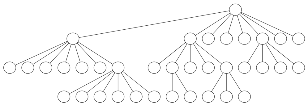
Figure 12 can help us visualize why this is so. The root of
the tree represents the starting point of the search. From there the
algorithm generates and checks each of the possible moves the knight can
make. As we have noted before, the number of moves possible depends on
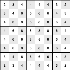
the position of the knight on the board. In the corners there are only
two legal moves, on the squares adjacent to the corners there are three,
and in the middle of the board there are eight. Figure 13
shows the number of moves possible for each position on a board. At the
next level of the tree there are once again between two and eight possible
next moves from the position we are currently exploring. The number of
possible positions to examine corresponds to the number of nodes in the
search tree.

Figure 12: A Search Tree for the Knight’s Tour

Figure 13: The Number of Possible Moves for Each Square
We have already seen that the number of nodes in a binary tree of height \(N\) is \(2^{N+1}-1\). For a tree with nodes that may have up to eight children instead of two, the number of nodes is much larger. Because the branching factor of each node is variable, we could estimate the number of nodes using an average branching factor. The important thing to note is that this algorithm is exponential: \(k^{N+1}-1\), where \(k\) is the average branching factor for the board. Let’s look at how rapidly this grows! For a board that is \(5 \times 5\) the tree will be 25 levels deep, or \(N = 24\) counting the first level as level 0. The average branching factor is \(k = 3.8\) so the number of nodes in the search tree is \(3.8^{25}-1\) or \(3.12 \times 10^{14}\). For a \(6 \times 6\) board, \(k = 4.4\), there are \(1.5 \times 10^{23}\) nodes, and for a regular \(8 \times 8\) chess board, \(k = 5.25\), there are \(1.3 \times 10^{46}\). Of course, since there are multiple solutions to the problem we won’t have to explore every single node, but the fractional part of the nodes we do have to explore is just a constant multiplier which does not change the exponential nature of the problem. We will leave it as an exercise for you to see if you can express \(k\) as a function of the board size.
Luckily there is a way to speed up the \(8 \times 8\) case so that it
runs in under one second. In the Listing 4 we show the code that
speeds up the knight_tour. This function, called order_by_avail,
will be used in place of the call to u.get_neighbors at line 8 in Listing 3.
The critical line in the
order_by_avail function is line 10. This line ensures that we select the vertex
that has the fewest available moves to go next. You
might think this is really counterproductive; why not select the node
that has the most available moves? You can try that approach easily by
running the program yourself and inserting the line
res_list.reverse() right after the sort.
The problem with using the vertex with the most available moves as your next vertex on the path is that it tends to have the knight visit the middle squares early on in the tour. When this happens it is easy for the knight to get stranded on one side of the board where it cannot reach unvisited squares on the other side of the board. On the other hand, visiting the squares with the fewest available moves first pushes the knight to visit the squares around the edges of the board first. This ensures that the knight will visit the hard-to-reach corners early and can use the middle squares to hop across the board only when necessary.
Utilizing this kind of knowledge to speed up an algorithm is called a heuristic. Humans use heuristics every day to help make decisions, and heuristic searches are often used in the field of artificial intelligence. This particular heuristic is called Warnsdorff’s algorithm, named after H. C. von Warnsdorff who published his idea in 1823.
Listing 4
 1def order_by_avail(n):
 2    res_list = []
 3    for v in n.get_neighbors():
 4        if v.color == "white":
 5            c = 0
 6            for w in v.get_neighbors():
 7                if w.color == "white":
 8                    c = c + 1
 9            res_list.append((c, v))
10    res_list.sort(key=lambda x: x[0])
11    return [y[1] for y in res_list]