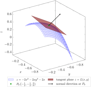
We can estimate the behavior of a function of two variables \(z = f(x,y)\) around a point \(P_0(x_0, y_0, f(x_0,y_0))\) by making the observation that the tangent plane to the surface \(z = f(x,y)\) at \(P_0\) can be used as such an approximation. Below is the formal definition.
Note that solving (8.2) for \(z\) gives exactly \(z = L(x,y)\text{:}\) the graph of the linearization is the tangent plane to the surface at \(P_0\text{.}\)
Consider the function \(f(x,y) = -2x^2 - 2xy^3 - 2x\text{.}\) Approximate \(f(x,y)\) near the point \(P_0\left(-0.5,\, -0.5,\, f(-0.5,-0.5)\right)\) with a linear function \(L(x,y)\text{.}\)
We use the equation of the tangent plane at \(P_0\left(-0.5, -0.5, f(-0.5,-0.5)\right)\) as a linear approximation for the surface, as follows. First we evaluate \(f\) and its partial derivatives at the point:
A blue mesh surface, the graph of z equals negative 2 x squared minus 2 x y cubed minus 2 x, seen close up around the point P 0. A flat dark red patch of the tangent plane z equals L of x y cuts through the mesh, touching it at the green point P 0 with coordinates negative one half, negative one half, three eighths: near P 0 the patch and the surface are indistinguishable, while away from P 0 the surface curves down and away from the flat patch. A long black arrow leaves P 0 at right angles to the patch, showing the normal direction to the surface there. A legend below the picture names the surface, the tangent plane, the point P 0, and the normal direction.
Figure8.10.The graph of \(z = -2x^2 - 2xy^3 - 2x\) and the tangent plane at \(P_0\left(-\frac12, -\frac12, \frac38\right)\text{,}\) whose equation is \(z = L(x,y) = \frac14\left(x+\frac12\right) +
\frac34\left(y+\frac12\right) + \frac38\text{.}\) The view is close in on \(P_0\text{,}\) where the plane hugs the surface, so that \(L(x,y)\) approximates \(f(x,y)\text{;}\) farther out the surface curves away from the plane. The arrow at \(P_0\) is the normal direction to the surface.