A. We begin by computing the normal vector to the surface at \(P_0(1,1,-2)\text{,}\) which is given by \(\mathbf n = \nabla w \Big|_{P_0}\text{,}\) where \(w(x,y,z) = -x^2 - y^2 - z\text{:}\)
\begin{align*}
\nabla w \amp= \left(\frac{\partial w}{\partial x}\right)\mathbf i
+ \left(\frac{\partial w}{\partial y}\right)\mathbf j
+ \left(\frac{\partial w}{\partial z}\right)\mathbf k\\
\amp= (-2x)\,\mathbf i + (-2y)\,\mathbf j + (-1)\,\mathbf k\\
\mathbf n \amp= \nabla w \Big|_{P_0}
= -2\,\mathbf i - 2\,\mathbf j - \mathbf k.
\end{align*}
Hence the parametric equations of the normal line are
B. Note that we have already calculated the normal vector \(\mathbf n = \langle -2, -2, -1 \rangle\) to the surface at \(P_0(1,1,-2)\text{,}\) and we are ready to write down the equation of the tangent plane:
\begin{align}
-2x - 2y - z \amp= D,\tag{8.12}\\
\text{where}\quad D \amp= \mathbf n \cdot \vec{OP_0}
= \langle -2, -2, -1 \rangle \cdot \langle 1, 1, -2 \rangle = -2.\notag
\end{align}
Therefore the tangent plane is
\begin{equation}
-2x - 2y - z = -2.\tag{8.13}
\end{equation}
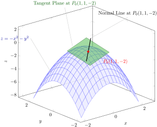
Figure 8.3 shows the surface, the tangent plane, and the normal line at \(P_0(1,1,-2)\text{.}\)
A downward-opening paraboloid drawn as a blue mesh, the graph of z equals negative x squared minus y squared. A green tangent plane patch touches the surface at the red point P 0 with coordinates 1, 1, negative 2, on the side of the dome. A black line passes through P 0 perpendicular to the plane: the normal line to the surface.
Figure8.3.The graph of \(z = -x^2 - y^2\text{,}\) the tangent plane \(-2x - 2y - z = -2\) (green), and the normal line \(x = 1-2t\text{,}\)\(y = 1-2t\text{,}\)\(z = -2-t\) (black) at the point \(P_0(1,1,-2)\text{.}\)
Figure 8.4 works through this computation from the start: it builds the gradient \(\nabla w\text{,}\) evaluates it at \(P_0\) to get the normal vector, and then draws the normal line and the tangent plane on the surface. Note that the video takes the normal vector in the outward direction, \(\mathbf n = -\nabla w \big|_{P_0} = \langle 2, 2, 1\rangle\text{,}\) which is the opposite of the \(\nabla w \big|_{P_0}\) used above; either choice gives the same normal line and the same tangent plane, since the two vectors differ only by the factor \(-1\text{.}\)
Figure8.4.Computing the normal vector for Example 8.2. The surface, the point \(P_0(1,1,-2)\text{,}\) the gradient computation, the normal vector, the normal line, and the tangent plane are built up in turn, followed by a slow rotation of the finished figure.