Flux Integrals

Section 12.9 Flux Integrals

Motivating Questions

How can we measure how much of a vector field flows through a surface in space?
🔗

🔗
How can we calculate the amount of a vector field that flows through common surfaces, such as the graph of a function $z = f (x, y) ?$
🔗

🔗

Section 11.6 showed how we can use vector valued functions of two variables to give a parameterization of a surface in space. For instance, the function

r (s, t) = ⟨ 2 \cos (t) \sin (s), 2 \sin (t) \sin (s), 2 \cos (s) ⟩

with domain

0 \leq t \leq 2 π

and

0 \leq s \leq π

parameterizes a sphere of radius

2

centered at the origin. Section 11.6 also gives examples of how to write parameterizations based on other geometric relationships like when one coordinate can be written as a function of the other two. In Subsection 11.6.2, we set up a Riemann sum based on a parameterization that would measure the surface area of our curved surfaces in space.

🔗

In Figure 12.9.1, we plot a surface using a parametrization

r (s, t) = ⟨ f (s, t), g (s, t), h (s, t) ⟩ .

The magenta curves represent curves where

s

varies and

t

is held constant, while the yellow curves represent curves where

t

varies and

s

is held constant. The vector in magenta is

r_{s} = \frac{\partial r}{\partial s} = ⟨ f_{s}, g_{s}, h_{s} ⟩

which measures the direction and magnitude of change in the coordinates of the surface when only

s

is varied. Similarly, the vector in yellow is

r_{t} = \frac{\partial r}{\partial t} = ⟨ f_{t}, g_{t}, h_{t} ⟩

which measures the direction and magnitude of change in the coordinates of the surface when only

t

is varied. We also plot the parallelogram that is formed by

r_{s}

and

r_{t},

which is tangent to the surface. The area of this parallelogram offers an approximation for the surface area of a patch of the surface.

🔗

Figure 12.9.1. A three-dimensional plot of Figure 11.6.6

🔗

From Section 9.4, we also know that

r_{s} \times r_{t}

(plotted in green) will be orthogonal to both

r_{s}

and

r_{t}

and its magnitude will be given by the area of the parallelogram.

🔗

Preview Activity 12.9.1.

In this preview activity, we will explore the parameterizations of a few familiar surfaces and confirm some of the geometric properties described in the introduction above.

🔗

(a)

Use the ideas from Section 11.6 to give a parameterization

r (s, t)

of the following surface. Be sure to specify the bounds on each of your parameters.

🔗

S_{1} :

the right circular cylinder centered on the

x

-axis of radius 2 when

0 \leq x \leq 5

🔗

(b)

Draw a graph of

S_{1}

from the previous part. Label the points that correspond to

(s, t)

points of

(0, 0),

(0, 1),

(1, 0),

and

(2, 3) .

🔗

(c)

For the parameterization from part a, calculate

r_{s},

r_{t},

and

r_{s} \times r_{t} .

🔗

(d)

For the parameterization from part a, find the value for

r_{s},

r_{t},

and

r_{s} \times r_{t}

at the

(s, t)

points of

(0, 0),

(0, 1),

(1, 0),

and

(2, 3) .

🔗

(e)

Draw your vector results from d on your graph and confirm the geometric properties described in the introduction to this section. Namely,

r_{s}

and

r_{t}

should be tangent to the surface, while

r_{s} \times r_{t}

should be orthogonal to the surface (in addition to

r_{s}

and

r_{t}

🔗

(f)

Repeat steps (a) through (e) for the following two surfaces:

🔗

(i)

S_{2} :

the sphere centered at the origin of radius 3

🔗

(ii)

S_{3} :

the first octant portion of the plane

x + 2 y + 3 z = 6

🔗

As we saw in Section 11.6, we can set up a Riemann sum of the areas for the parallelograms in Figure 12.9.1 to approximate the surface area of the region plotted by our parametrization. Equation (11.6.2) shows that we can compute the exact surface area by taking a limit of a Riemann sum which will correspond to integrating the magnitude of

r_{s} \times r_{t}

over the appropriate parameter bounds. What if we wanted to measure a quantity other than the surface area? Our focus in this section we will be the exploration of a specific case of this question: How can we measure the amount of a three dimensional vector field that flows through a particular section of a surface? The geometric tools we have reviewed in this section, especially the vector

r_{s} \times r_{t},

will be valuable.

🔗

Subsection 12.9.1 The Idea of the Flux of a Vector Field through a Surface

In this section we will look at how to measure the amount of a vector field that flows through a surface in space. Figure 12.9.2 illustrates a plot that demonstrates this idea. Our definition of divergence in Section 12.6 looked at measuring the amount of vector field flowing out of a small region on a 2D plane. In this subsection, we will set up a precise measurement of this same measurement but over a region of a curved surface in 3D.

🔗

Figure 12.9.2. A three-dimensional vector field and a surface

🔗

As with understanding line integrals of vector-valued functions in Section 12.2, we don’t care about the output of the vector field at points away from the surface. We would really would like to examine the output vectors for the points on our surface. To do this, we will look at Figure 12.9.3, which plots the output of our vector field at an array of points on our surface.

🔗

Figure 12.9.3. A three-dimensional vector field evaluated along a surface

🔗

The central question we would like to consider is “How can we measure the amount of a three dimensional vector field that flows through a particular section of a curved surface?”, so we only need to consider the amount of the vector field that flows through the surface. Any portion of our vector field that flows along (or tangent) to the surface will not contribute to the amount that goes through the surface. In Figure 12.9.4, we have split the vector field for points on our surface into two components. One component, plotted in green, is orthogonal to the surface. The component that is tangent to the surface is plotted in magenta.

🔗

Figure 12.9.4. The decomposition of three-dimensional vector field evaluated along a surface into normal and tangent components

🔗

In order to measure the amount of the vector field that moves through the plotted section of the surface, we must find the accumulation of the lengths of the green vectors in Figure 12.9.4. Notice that some of the green vectors are moving through the surface in a direction opposite of others. In other words, we will need to pay attention to the direction in which these vectors move through our surface and not just the magnitude of the green vectors.

🔗

If we have a parameterization of the surface, then the vector

r_{s} \times r_{t}

varies smoothly across our surface and gives a consistent way to describe which direction we choose as “through” the surface. If we define a positive flow through our surface as being consistent with the yellow vector in Figure 12.9.4, then there is more positive flow (in terms of both magnitude and area) than negative flow through the surface. Thus, the net flow of the vector field through this surface is positive.

🔗

Activity 12.9.2. Visualizing flux through a surface.

In this activity, you will compare the net flow of different vector fields through our sample surface. In Figure 12.9.5 you can select between five different vector fields. Once you select a vector field, the vector field for a set of points on the surface will be plotted in blue. Each blue vector will also be split into its normal component (in green) and its tangential component (in magenta). The yellow vector defines the direction for positive flow through the surface.

🔗

Look at each vector field and order the vector fields from greatest net flow through the surface to least net flow through the surface. Remember that a negative net flow through the surface should be lower in your rankings than any positive net flow.

🔗

Figure 12.9.5. Five vector fields flowing through a surface, with decomposition into normal and tangential components

🔗

Subsection 12.9.2 The Details of Measuring the Flux of a Vector Field through a Surface

Now that we have developed a conceptual understanding of what we are trying to measure, we can set up the corresponding Riemann sum to measure the flux of a vector field through a section of a surface. Let

Q

be the section of our surface and suppose that

Q

is parameterized by

r (s, t)

with

a \leq s \leq b

and

c \leq t \leq d .

The domain of

r

is a region of the

s t

-plane, which we call

D,

and the range of

r

Q .

🔗

As with most problems in integral calculus, we slice our region of interest into smaller pieces. Specifically, we slice

a \leq s \leq b

into

n

equally-sized subintervals with endpoints

s_{0}, s_{1}, \dots, s_{n}

and

c \leq t \leq d

into

m

equally-sized subintervals with endpoints

t_{0}, t_{1}, \dots, t_{n} .

This divides

D

into

n m

rectangles of size

Δ s = \frac{b - a}{n}

Δ t = \frac{d - c}{m} .

We index these rectangles as

D_{i, j} .

Every

D_{i, j}

has area (in the

s t

-plane)

Δ s Δ t .

The partition of

D

into the rectangles

D_{i, j}

also partitions

Q

into

n m

corresponding pieces which we call

Q_{i, j} = r (D_{i, j}) .

From Section 11.6 (specifically (11.6.1)) the surface area of

Q_{i, j}

is approximated by

S_{i, j} = | (r_{s} \times r_{t}) (s_{i}, t_{j}) | Δ s Δ t .

🔗

Figure 12.9.6. Pieces of the tangent planes that approximate a surface

🔗

We want to measure the total flow of the vector field

F

through

Q,

which we will approximate on each

Q_{i, j}

and then sum to obtain the total flow. In other words, the flux of

F

through

Q

Flux = \sum_{i = 1}^{n} \sum_{j = 1}^{m} | F_{⊥ Q_{i, j}} | \cdot S_{i, j},

where

| F_{⊥ Q_{i, j}} |

is the length of the component of

F

orthogonal to

Q_{i, j} .

🔗

For each

Q_{i, j},

we approximate the surface

Q

by the tangent plane to

Q

at a corner of that partition element. This corresponds to using the planar elements in Figure 12.9.6, which have surface area

S_{i, j} .

The vector

w_{i, j} = (r_{s} \times r_{t}) (s_{i}, t_{j})

can be used to measure the orthogonal direction (and thus define which direction we mean by positive flow through

Q

) on the

i, j

partition element. This means that

F_{⊥ Q_{i, j}} = | {proj}_{w_{i, j}} F (s_{i}, t_{j}) | = \frac{F (s_{i}, t_{j}) \cdot w_{i, j}}{| w_{i, j} |}

🔗

Combining these pieces, we find that the flux through

Q_{i, j}

is approximated by

\begin{aligned} Flux through Q_{i, j} & = | F_{⊥ Q_{i, j}} | \cdot S_{i, j} = (\frac{F_{i, j} \cdot w_{i, j}}{| w_{i, j} |}) (| w_{i, j} | Δ s Δ t) \\ = (F_{i, j} \cdot (r_{s} \times r_{t})) (Δ s Δ t), \end{aligned}

where

F_{i, j} = F (s_{i}, t_{j}) .

Therefore we may approximate the total flux by

Total Flux = \sum_{i = 1}^{n} \sum_{j = 1}^{m} (F_{i, j} \cdot w_{i, j}) (Δ s Δ t) .

Taking the limit as

n, m \to \infty

gives the following result.

🔗

Conceptually, the above limit shows how the argument in Subsection 11.6.2 generalizes when measuring the flux of a vector field through a surface rather than just the surface area. The key difference between the Riemann sum above and Riemann sum used to set up Surface area is that we are using the dot product of the vector field with the normal vector to the surface (given by

w_{i, j} = (r_{s} \times r_{t}) (s_{i}, t_{j})

) as the scalar value in our sum. This realization gives the following theorem, which states that the flux through a curved surface in space can be computed using a parameterization of the surface and a double integral over a flat region in the plane of parameter values.

🔗

Theorem 12.9.7.

Let a smooth surface

Q

be parametrized by

r (s, t)

over a domain

D .

The total flux of a smooth vector field

F

through

Q

is given by

\iint_{D} F \cdot (r_{s} \times r_{t}) d A .

🔗

In Figure 12.9.6, you can change the number of sections in the partition and see the geometric result of refining the partition. In the next example, we will look at how Theorem 12.9.7 is used on a part of a cone and make sense of the vector

w (t, s) = r_{s} \times r_{t}

and the scalar

F \cdot (r_{s} \times r_{t}) .

🔗

Remark 12.9.8.

In some Webwork exercises and other sources, you will see flux integrals specified with the following notations:

\iint_{S_{1}} F \cdot (r_{s} \times r_{t}) d A = \iint_{S_{1}} F \cdot d \vec{A} = \iint_{S_{1}} F \cdot d \vec{S}

While we will use the notation specified in Theorem 12.9.7 primarily, the other notations come from combining the normal vector (calculated from the parameterization of the surface) and the area element into a single vector valued area element. In other words,

(r_{s} \times r_{t}) d A = d \vec{A} = d \vec{s} .

🔗

Example 12.9.9.

In this example we will compute the flux of the vector field

F = ⟨ x z - 2, y + x, 1 ⟩

through the surface of the cone given by

x^{2} + y^{2} = z^{2}

with

1 \leq z \leq 3 .

So that we can use Theorem 12.9.7, we first parameterize our surface and calculate

w (t, s) = r_{s} \times r_{t}

based on that parameterization.

🔗

In cylindrical coordinates, our cone is described by

r = z

which suggests that we can use

r

and

θ

s

and

t .

Consider the parameterization

r (s, t) = ⟨ s \cos (t), s \sin (t), s ⟩

with bounds

1 \leq s \leq 3

and

0 \leq t < 2 π .

Notice that

s

is acting as both

r

and

z .

Calculating the partial derivatives of

r

gives the following:

\begin{aligned} r_{s} & = ⟨ \cos (t), \sin (t), 1 ⟩ \\ r_{t} & = ⟨ - s \sin (t), s \cos (t), 0 ⟩ \end{aligned}

Taking the cross product of

r_{s}

and

r_{t},

we obtain the vector-valued function

w :

w = r_{s} \times r_{t} = ⟨ - s \cos (t), - s \sin (t), s (\cos (t)^{2} + \sin (t)^{2}) ⟩ .

We may simplify this to

w = ⟨ - s \cos (t), - s \sin (t), s ⟩ .

Notice that

w

is very close to

r .

If we think of

r

as giving

⟨ x, y, z ⟩,

then

w = ⟨ - x, - y, z ⟩ .

The figure below shows the relationship between vectors

r

and

w

for a point on the surface.

🔗

Figure 12.9.10. A plot of our surface with the parameterization vector in green and the normal vector

w

in magenta

🔗

In Figure 12.9.10, the normal vector (as calculated from the parameterization) points inside the cone. This is the direction of positive flow when measuring the flux of the vector field. Our parameterization will also transform our vector field into a function of

s

and

t .

Specifically,

F (s, t) = ⟨ (s \cos (t)) (s) - 2, s \sin (t) + s \cos (t), 1 ⟩

Applying Theorem 12.9.7 to our parameterization and vector field allows us to compute

I = \iint_{D} F \cdot (r_{s} \times r_{t}) d A

as an interated integral

\begin{aligned} I & = \int_{0}^{2 π} \int_{1}^{3} ⟨ (s \cos (t)) (s) - 2, s \sin (t) + s \cos (t), 1 ⟩ \cdot ⟨ - s \cos (t), - s \sin (t), s ⟩ d s d t \\ = \int_{0}^{2 π} \int_{1}^{3} ((s \cos (t)) (s) - 2) (- s \cos (t)) + (- s \sin (t)) (s \sin (t) + s \cos (t)) + s \\ = - \frac{62}{3} π . \end{aligned}

Note that the result of this flux integral is negative, which means more of the vector field is going out of the cone than is coming into the cone.

🔗

Figure 12.9.11. A plot of the surface with the vector field

F

for an array of points on the surface. The vector field has been scaled down by a factor of 5 in this plot.

🔗

In Figure 12.9.11 you can see much more of the vector field is flowing outside of the cone than inside, which matches with our result of calculating the flux as negative.

🔗

The next activity asks you to carefully go through the process of calculating the flux of some vector fields through a cylindrical surface.

🔗

Activity 12.9.3. Checking the Visualization for Flux.

(a)

Figure 12.9.12 shows a plot of the vector field

F = ⟨ y, z, 2 + \sin (x) ⟩

and a right circular cylinder of radius

2

and height

3

(with open top and bottom). Consider the vector field going into the cylinder (toward the

z

-axis) as corresponding to positive flux.

🔗

Figure 12.9.12. The vector field

F = ⟨ y, z, 2 + \sin (x) ⟩

and a right circular cylinder

🔗

(i)

Reasoning graphically, do you think the flux of

F

throught the cylinder will be positive, negative, or zero? Write a few sentences jutifying your answer.

🔗

(ii)

Parameterize the right circular cylinder of radius

2,

centered on the

z

-axis, for

0 \leq z \leq 3 .

Be sure to give bounds on your parameters.

🔗

(iii)

Based on your parameterization, compute

r_{s},

r_{t},

and

r_{s} \times r_{t} .

Confirm that these vectors are either orthogonal or tangent to the right circular cylinder. Is your orthogonal vector pointing in the direction of positive flux or negative flux?

🔗

(iv)

Use your parametrization to write

F

as a function of

s

and

t .

🔗

Hint.

The

x

-coordinate is given by the first component of

r .

🔗

(v)

Compute the flux of

F

through the parameterized portion of the right circular cylinder.

🔗

(vi)

Does your computed value for the flux match your prediction from earlier?

🔗

(vii)

Use Figure 12.9.13 to make an argument about why the flux of

F = ⟨ y, z, 2 + \sin (x) ⟩

through the right circular cylinder is zero.

🔗

Figure 12.9.13. The vector field

F = ⟨ y, z, 2 + \sin (x) ⟩

with normal and tangential components plotted on a right circular cylinder

🔗

(b)

Write a couple of sentences to explalin how the results of the flux calculations would be different if we used the vector field

F = ⟨ y, z, \cos (x y) + \frac{9}{z^{2} + 6.2} ⟩

and the same right circular cylinder.

🔗

(c)

write a couple of sentences to explain how the results of the flux calculations would be different if we used the vector field

F = ⟨ y, - x, 3 ⟩

and the same right circular cylinder.

🔗

In the exercises for this section, we will look at some computational ideas to help us more efficiently compute the value of a flux integral. In many cases, the surface we are looking at the flux through can be written with one coordinate as a function of the others. For simplicity, we consider

z = f (x, y) .

Additionally, there will be exercises that guide you through common surfaces like spheres and cylinder surfaces.

🔗

Remark 12.9.14.

Note that throughout this section, we have implicitly assumed that we can parametrize the surface

S

in such a way that

r_{s} \times r_{t}

gives a well-defined normal vector. Technically, this means that the surface be orientable. Most “reasonable” surfaces are orientable. However, there are surfaces that are not orientable. Perhaps the most famous is formed by taking a long, narrow piece of paper, giving one end a half twist, and then gluing the ends together. Try doing this yourself, but before you twist and glue (or tape), poke a tiny hole through the paper on the line halfway between the long edges of your strip of paper and circle your hole. After gluing, place a pencil with its eraser end on your dot and the tip pointing away. Think of this as a potential normal vector. Keep the eraser on the paper, and follow the middle of your surface around until the first time the eraser is again on the dot. Is your pencil still pointing the same direction relative to the surface that it was before?

🔗

Subsection 12.9.3 Summary

A flux integral of a vector field, $F,$ on a surface in space, $S,$ measures how much of $F$ goes through $S_{1} .$
🔗

🔗
Let the smooth surface, $S,$ be parametrized by $r (s, t)$ over a domain $D .$ The total flux of a smooth vector field $F$ through $S$ is given by

$\iint_{D} F \cdot (r_{s} \times r_{t}) d A .$

🔗

🔗
If $S_{1}$ is of the form $z = f (x, y)$ over a domain $D,$ then the total flux of a smooth vector field $F$ through $S_{1}$ is given by

$\iint_{D} F (x, y, f (x, y)) \cdot ⟨ - \frac{\partial f}{\partial x}, - \frac{\partial f}{\partial y}, 1 ⟩ d A .$

🔗

🔗

🔗

Exercises 12.9.4 Exercises

1.

Compute the flux of the vector field

\vec{v} = - 4 \vec{i} - 5 \vec{j} - 4 \vec{k}

through the rectangular region shown below, assuming it is oriented as shown and that

a = 2

and

b = 4 .

🔗

flux =

🔗

2.

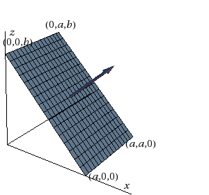
Calculate the flux of the vector field

\vec{F} (x, y, z) = 3 y \vec{j}

through a square of side length

7

in the plane

y = 6 .

The square is centered on the y-axis, has sides parallel to the axes, and is oriented in the positive y-direction.

🔗

Flux =

🔗

Hint.

y = 6 .

🔗

3.

(a) Set up a double integral for calculating the flux of the vector field

\vec{F} (x, y, z) = z^{2} \vec{k}

through the upper hemisphere of the sphere

x^{2} + y^{2} + z^{2} = 9,

oriented away from the origin. If necessary, enter

ρ

as rho,

θ

as theta, and

ϕ

as phi.

🔗

Flux =

\int_{A}^{B} \int_{C}^{D}

d ϕ d θ

A =

B =

C =

D =

(b) Evaluate the integral.

🔗

Flux =

\iint_{S} \vec{F} \cdot d \vec{A}

🔗

Hint.

z = ρ \cos (ϕ) .

🔗

4.

Compute the flux of the vector field

\vec{F} = 5 x^{2} y^{2} z \vec{k}

through the surface

S

which is the cone

\sqrt{x^{2} + y^{2}} = z,

with

0 \leq z \leq R,

oriented downward.

🔗

(a) Parameterize the cone using cylindrical coordinates (write

θ

as theta).

🔗

x (r, θ) =

🔗

y (r, θ) =

🔗

z (r, θ) =

🔗

with

\leq r \leq

🔗

and

\leq θ \leq

🔗

(b) With this parameterization, what is

d \vec{A} ?

🔗

d \vec{A}

🔗

(c) Find the flux of

\vec{F}

through

S .

🔗

flux =

🔗

5.

Compute the flux of the vector field

\vec{F} = z \vec{i} + 6 x \vec{j}

through the parameterized surface

S

oriented upward and given, for

0 \leq s \leq 3, 2 \leq t \leq 3,

x = s^{2}, y = 2 s + t^{2}, z = 5 t .

🔗

flux =

🔗

6.

Are the following statements true or false?

🔗

If $S_{1}$ is a rectangle with area 1 and $S_{2}$ is a rectangle with area 2, then $2 \iint_{S_{1}} \vec{F} \cdot d \vec{A} = \iint_{S_{2}} \vec{F} \cdot d \vec{A}$
🔗

🔗
The area vector of a flat, oriented surface is parallel to the surface.
🔗

🔗
If $S$ is the unit sphere centered at the origin, oriented outward and $\vec{F} = x \vec{i} + y \vec{j} + z \vec{k} = \vec{r},$ then the flux integral $\iint_{S} \vec{F} \cdot d \vec{A}$ is positive.
🔗

🔗
If $S$ is the unit sphere centered at the origin, oriented outward and the flux integral $\iint_{S} \vec{F} \cdot d \vec{A}$ is zero, then $\vec{F} (x, y, z)$ is perpendicular to $\vec{r} = ⟨ x, y, z ⟩$ at every point of $S .$
🔗

🔗
If $S$ is the unit sphere centered at the origin, oriented outward and the flux integral $\iint_{S} \vec{F} \cdot d \vec{A}$ is zero, then $\vec{F} = \vec{0} .$
🔗

🔗
If $S$ is an open-ended circular cylinder centered about the z-axis, oriented away from the z-axis, and $\vec{F} = ⟨ x, y, 0 ⟩,$ then the flux of $\vec{F}$ through $S$ is positive.
🔗

🔗
If $S$ is an open-ended circular cylinder centered about the z-axis, oriented away from the z-axis, and $\vec{F} = ⟨ 3, - 2, 6 ⟩,$ then the flux of $\vec{F}$ through $S$ is zero.
🔗

🔗
If $S$ is the cube bounded by the six planes $x = \pm 3,$ $y = \pm 3,$ $z = \pm 3,$ oriented outward, and $\vec{F} = 2 \vec{i} - \vec{k},$ then the flux of $\vec{F}$ through $S$ is zero.
🔗

🔗

🔗

7.

Let

S

be the square in the

x y

-plane shown in the figure below, oriented with the normal pointing in the positive

z

-direction. Estimate

\iint_{S} F \cdot d S

where

F

is a vector field whose values at the labeled points are

\begin{array}{llll} F (A) & = ⟨ 5, 8, 3 ⟩, & F (B) & = ⟨ - 6, 6, - 9 ⟩ \\ F (C) & = ⟨ - 4, - 9, - 6 ⟩, & F (D) & = ⟨ - 1, 2, - 6 ⟩ \end{array}

🔗

\iint_{S} F \cdot d S \approx

🔗

8.

F =

x i + y j + 5 z k

and

σ

is the portion of the cone

z = \sqrt{x^{2} + y^{2}}

between the planes

z = 5

and

z = 10

oriented with normal vectors pointing upwards. Find the flux of the flow field F across

σ :

🔗

9. Flux Through Surfaces of the Form $z = f (x, y)$ .

In this exercise, we will look at how to use a parametrization of a surface that can be described as

z = f (x, y)

to efficiently calculate flux integrals.

🔗

(a)

Suppose that

S

is a surface given by

z = f (x, y) .

Find a parametrization

r (s, t)

S .

🔗

Hint.

Use

s = x

and

t = y .

🔗

(b)

Show that the vector orthogonal to the surface

S

has the form

r_{s} \times r_{t} = ⟨ - \frac{\partial f}{\partial x}, - \frac{\partial f}{\partial y}, 1 ⟩ .

🔗

(c)

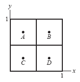
For each of the three surfaces given below, compute

r_{s} \times r_{t},

graph the surface, and compute

r_{s} \times r_{t}

for four different points of your choosing. You should make sure your vectors

r_{s} \times r_{t}

are orthogonal to your surface.

🔗

(i)

z = x^{2} + y^{2}

🔗

(ii)

x + 2 y + z = - 4

🔗

(iii)

z = x^{2} - y^{2}

🔗

(d)

For each of the three surfaces in part c, use your calculations and Theorem 12.9.7 to compute the flux of each of the following vector fields through the part of the surface corresponding to the region

D

in the

x y

-plane.

🔗

(i)

F = ⟨ x, y, z ⟩

with

D

given by

0 \leq x, y \leq 2

🔗

(ii)

F = ⟨ - y, x, 1 ⟩

with

D

as the triangular region of the

x y

-plane with vertices

(0, 0),

(1, 0),

and

(1, 1)

🔗

(iii)

F = ⟨ z, y - x, (y - x)^{2} - z^{2} ⟩

with

D

given by

0 \leq x, y \leq 2

🔗

10. Calculating the Flux through a Sphere.

For this activity, let

S_{R}

be the sphere of radius

R

centered at the origin.

🔗

(a)

Parametrize

S_{R}

using spherical coordinates. Give your parametrization as

r (s, t),

and be sure to state the bounds of your parametrization.

🔗

Hint.

Use

s = θ

and

t = ϕ .

🔗

(b)

Use your parametrization of

S_{R}

to compute

r_{s} \times r_{t} .

🔗

(c)

Your result for

r_{s} \times r_{t}

should be a scalar expression times

r (s, t) .

Explain why the outward pointing orthogonal vector on the sphere is a multiple of

r (s, t)

and what that scalar expression means.

🔗

(d)

Use your parametrization of

S_{2}

and the results of part b to calculate the flux through

S_{2}

for each of the three following vector fields.

🔗

(i)

F_{1} = ⟨ x, y, z ⟩

🔗

(ii)

F_{2} = ⟨ - y, x, - 1 ⟩

🔗

(iii)

F_{3} = ⟨ x - y, y + x, z - 1 ⟩

🔗

(e)

Use computer software to plot each of the vector fields from part d and interpret the results of your flux integral calculations.

🔗

(f)

If we used the sphere of radius 4 instead of

S_{2},

explain how each of the flux integrals from part d would change. You do not need to calculate these new flux integrals, but rather explain if the result would be different and how the result would be different.

🔗

Subsection 12.9.5 Notes to Instructors and Dependencies

This section relies on parameterized surfaces, which was first introduced in Section 11.6. While some of the activities in this section may be too much for a single student to do in a class setting, we suggest that different cases of the vector fields and surfaces can be split for small group work. Students can then present answers to the larger group.

🔗

You have attempted 1 of 9 activities on this page.

🔗

Prev Top Next

Section 12.9 Flux Integrals

Motivating Questions

Preview Activity 12.9.1.

(a)

(b)

(c)

(d)

(e)

(f)

(i)

(ii)

Subsection 12.9.1 The Idea of the Flux of a Vector Field through a Surface

Activity 12.9.2. Visualizing flux through a surface.

Subsection 12.9.2 The Details of Measuring the Flux of a Vector Field through a Surface

Theorem 12.9.7.

Remark 12.9.8.

Example 12.9.9.

Activity 12.9.3. Checking the Visualization for Flux.

(a)

(i)

(ii)

(iii)

(iv)

(v)

(vi)

(vii)

(b)

(c)

Remark 12.9.14.

Subsection 12.9.3 Summary

Exercises 12.9.4 Exercises

1.

2.

3.

4.

5.

6.

7.

8.

9. Flux Through Surfaces of the Form z=f(x,y).

(a)

(b)

(c)

(i)

(ii)

(iii)

(d)

(i)

(ii)

(iii)

10. Calculating the Flux through a Sphere.

(a)

(b)

(c)

(d)

(i)

(ii)

(iii)

(e)

(f)

Subsection 12.9.5 Notes to Instructors and Dependencies

9. Flux Through Surfaces of the Form $z = f (x, y)$ .