Outliers and Skew
What would happen if you drastically altered one of the data points in a dataset? For example, if you rolled a dice where the value of 6 is replaced by 60? How does adding such a value, called an outlier, affect the different measures of center?
Outlier Definition
An outlier is a data point that is significantly far away from most other data points. For example, if everyone in your classroom is of average height with the exception of two basketball players that are significantly taller than the rest of the class, these two data points would be considered outliers.
Outliers in a Histogram
Consider the histogram of student heights below.
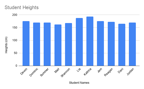
In this example, there are two students whose heights are much greater than the rest of the students. Lia’s height is 188 centimeters (cm) and Katrina’s height is 193 cm. Taking the mean of the students’ heights results in 168.45 cm.
Using the mean as the only summary statistic of a dataset can often be misleading. For example, consider the effects if this school decided to use the mean to decide how high the student desks needed to be. This would result in desks that are too high for most students, but too small for Lia and Katrina.
Skew Definition
Skewness is a measure of asymmetry of a dataset. For example, a dataset has a skew if there are values far away from the mean on one side (either above or below), but far fewer values the same distance from the mean on the other side. A positive skew occurs when the dataset contains values much greater than the mean but far fewer values less than the mean. A negative skew occurs when the dataset contains values much less than the mean but far fewer values much greater than the mean.
Outliers and skew only pertain to quantitative variables. (For categorical variables, there is no notion of “distance” between different categories.)
Skew in a Histogram
Consider the histogram of average exam scores below.
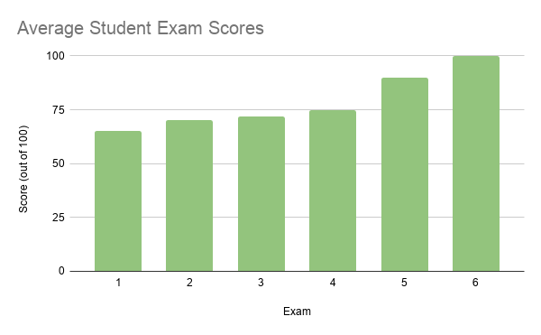
This is an example of negative skew. The mean is 81, and there are a large number of values that are lower than 81. This large group of values below the mean is called a left tail, and as such a negative skew is often called a left skew. Similarly, a dataset with a positive skew looks like a mirror image of the histogram above, with a right tail and a right skew.
Example: Positive Skew
Consider the histogram of a variable below.
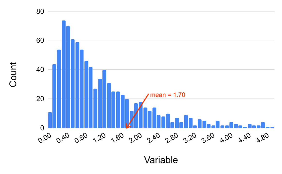
While most of the data lies in the interval between 0 and 1.5, there are values in the dataset that are much higher (but none that are below 0). This is an example of a positive skew. An example of a real dataset that might look like the histogram above is outlined below.
Q-1: What real-world variable do you think could have the histogram above?
Q-2: In the histogram above, do you think more of the values are above or below the mean? How does that compare to the median? Will the median be greater or less than the mean in this case?
Q-3: Find some examples of variables with left skew. Are there more data points above or below the mean? How does the mean compare to the median?
Example: Dice Roll
Outliers have different effects on different statistics. For example, if you change the 6 on a dice to 60, the minimum value of the roll is still 1, while the maximum value is now 60.
Outliers also have different effects on different measures of center. See what happens to the mean and median for the dice roll when the 6 is changed to a 60.
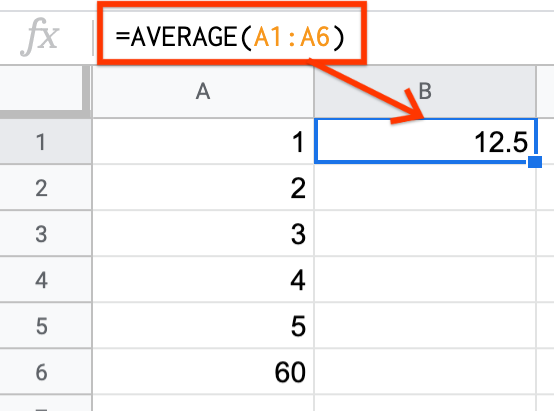
The mean of the dice roll is now 12.5! Only one value was changed, yet the mean changed drastically.
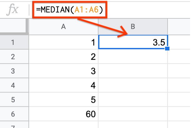
In contrast, the median does not change at all. The median is considered more “robust to outliers” than the mean. This means that as extreme values become more extreme or as outliers are introduced into the dataset, the median is less likely than the mean to be substantially affected.
Q-4: What would happen to the mean and median if you change the 1 of a standard dice to -10? What about if you change the 3 to 300?
Example: Income
Medians are especially useful when a dataset tends to lean towards higher/lower values. This is called a skew. Consider the example of income that has already been explored. Income is an extremely skewed dataset. You can read more about the income distribution here.
The following is an excerpt from the US census report on income from 2003.
“The distribution of wealth in the United States has a large positive skew, with relatively few households holding a large proportion of the wealth. For this type of distribution, the median is the preferred measure of central tendency because it is less sensitive than the average (mean) to extreme observations. The median is also considerably lower than the average, and provides a more accurate representation of the wealth and asset holdings of the typical household. For example, more households have a net worth near the median of $55,000 than near the average of $182,381.”
Since there are some households that earn extremely high incomes, just these few values can affect the mean too much (in the same way that changing 6 to 60 affected the mean for the dice roll). The median is preferred in such contexts.
Further Application
In the real world, skew is present in many different fields, including economics. For more information about how skew affects financial markets, see this article on skewness in finance.