ORCCA Graphs and Equations Chapter Review

Section 13.8 Graphs and Equations Chapter Review

Subsection 13.8.1 Overview of Graphing

In Section 1 we reviewed several ways of making graphs of both lines (by hand) and general functions (using technology).

🔗

Example 13.8.1. Graphing Lines by Plotting Points.

Graph the equation

y = \frac{5}{3} x - 3

by creating a table of values and plotting those points.

🔗

Explanation.

To make a good table for this line, we should have

x

-values that are multiples of

3

to make sure that the fraction cancels nicely for the outputs.

$x$	$y = \frac{5}{3} x - 3$	Point
$- 3$	$\frac{5}{3} (- 3) - 3 = - 8$	$(1, - 8)$
$0$	$\frac{5}{3} (0) - 3 = - 3$	$(2, - 3)$
$3$	$\frac{5}{3} (3) - 3 = 2$	$(3, 2)$
$6$	$\frac{5}{3} (6) - 3 = 7$	$(4, 7)$

Figure 13.8.2. A table of values for

y = \frac{5}{3} x - 3

Figure 13.8.3. A graph of

y = \frac{5}{3} x - 3

🔗

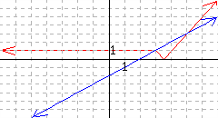
Example 13.8.4. Graphing Lines in Slope-Intercept Form.

Find the slope and vertical intercept of

j (x) = - \frac{7}{2} x + 5,

and then use slope triangles to find the next two points on the line. Draw the line.

🔗

Explanation.

The slope of

j (x) = - \frac{7}{2} x + 5

- \frac{7}{2},

and the vertical intercept is

(0, 5) .

Starting at

(0, 5),

we go down

7

units and right

2

units to reach more points.

From the graph, we can read that two more points that

j (x) = - \frac{7}{2} x + 5

passes through are

(2, - 2)

and

(4, 9) .

Figure 13.8.5. A graph of

j (x) = - \frac{7}{2} x + 5

🔗

Example 13.8.6. Graphing Lines in Point-Slope Form.

From the equation, find the slope and a point on the graph of

k (x) = \frac{3}{4} (x - 2) - 5,

and then use slope triangles to find the next two points on the line. Draw the line.

🔗

Explanation.

The slope of

k (x) = \frac{3}{4} (x - 2) - 5

\frac{3}{4}

and the point on the graph given in the equation is

(2, - 5) .

So to graph

k,

start at

(2, - 5),

and the go up

3

units and right

4

units (or down

3

left

4

) to reach more points.

From the graph, we can read that two more points that

k (x) = \frac{3}{4} (x - 2) - 5

passes through are

(6, - 2)

and

(10, 1) .

Figure 13.8.7. A graph of

k (x) = \frac{3}{4} (x - 2) - 5

🔗

Example 13.8.8. Graphing Lines Using Intercepts.

Use the intercepts of

4 x - 2 y = 16

to graph the equation.

🔗

Explanation.

To find the

x

-intercept, set

y = 0

and solve for

x .

\begin{aligned} 4 x - 2 (0) & = 16 \\ 4 x & = 16 \\ x & = 4 \end{aligned}

The

x

-intercept is the point

(4, 0) .

To find the

y

-intercept, set

x = 0

and solve for

y .

\begin{aligned} 4 (0) - 2 y & = 16 \\ - 2 y & = 16 \\ y & = - 8 \end{aligned}

The

y

-intercept is the point

(0, - 8) .

Next, we just plot these points and draw the line that runs through them.

Figure 13.8.9. A graph of

4 x - 2 y = 16

🔗

Example 13.8.10. Graphing Functions by Plotting Points.

The wind chill

en.wikipedia.org/wiki/Wind_chill

is how cold it feels outside due to the wind. Imagine a chilly 32 °F day with a breeze blowing over the snowy ground. The wind chill,

w (v),

at this temperature can be approximated by the formula

w (v) = 54.5 - 21 \sqrt[6]{v}

where

v

is the speed of the wind in miles per hour. This formula only approximates the wind chill for reasonable wind values of about 5 mph to 60 mph. Create a table of values rounded to the nearest tenth for the wind chill at realistic wind speeds and make a graph of

w .

🔗

Explanation.

Typical wind speeds vary between

5

and 20 mph, with gusty conditions up to 60 mph, depending on location. A good way to enter the sixth root into a calculator is to recall that

\sqrt[6]{x} = x^{\frac{1}{6}} .

$v$	$w (v) = 54.5 - 21 \sqrt[6]{v}$	Point	Interpretation
$5$	$w (5) \approx 27.0$	$(5, 27.0)$	A 5 mph wind causes a wind chill of 27.0 °F.
$10$	$w (10) \approx 23.7$	$(10, 23.7)$	A 10 mph wind causes a wind chill of 23.7 °F.
$20$	$w (20) \approx 19.9$	$(20, 19.9)$	A 20 mph wind causes a wind chill of 19.9 °F.
$30$	$w (30) \approx 17.5$	$(30, 17.5)$	A 30 mph wind causes a wind chill of 17.5 °F.
$40$	$w (40) \approx 15.7$	$(40, 15.7)$	A 40 mph wind causes a wind chill of 15.7 °F.
$50$	$w (50) \approx 14.2$	$(50, 14.2)$	A 50 mph wind causes a wind chill of 14.2 °F.
$60$	$w (60) \approx 12.9$	$(60, 12.9)$	A 60 mph wind causes a wind chill of 12.9 °F.

Figure 13.8.11. A table of values for

w (v) = 54.5 - 21 \sqrt[6]{v}

With the values in Table 11, we can sketch the graph.

the graph of the curve w(v)=54.5 - 21 times the sixth root of v — Figure 13.8.12. A graph of $w (v) = 54.5 - 21 \sqrt[6]{v}$

🔗

Subsection 13.8.2 Quadratic Graphs and Vertex Form

In Section 2 we covered the use of technology in analyzing quadratic functions, the vertex form of a quadratic function and how it affects horizontal and vertical shifts of the graph of a parabola, and the factored form of a quadratic function.

🔗

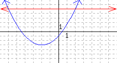
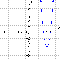
Example 13.8.13. Exploring Quadratic Functions with Graphing Technology.

Use technology to graph and make a table of the quadratic function

g

defined by

g (x) = - x^{2} + 5 x - 6

and find each of the key points or features.

🔗

Find the vertex.
Find the vertical intercept.
Find the horizontal intercept(s).
Find $g (- 1) .$
Solve $g (x) = - 6$ using the graph.
Solve $g (x) \leq - 6$ using the graph.
State the domain and range of the function.

🔗

Explanation.

The specifics of how to use any one particular technology tool vary. Whether you use an app, a physical calculator, or something else, a table and graph should look like:

$x$	$g (x)$
$- 1$	$- 12$
$0$	$- 6$
$1$	$- 2$
$2$	$0$
$2$	$0$
$3$	$0$
$4$	$- 2$

$the graph of the parabola g(x)=-x^2+5x-6, that opens downward, passing through the points listed in the table$

Additional features of your technology tool can enhance the graph to help answer these questions. You may be able to make the graph appear like:

$the previous graph with all of the key points labeled as described below$

The vertex is $(2.5, 0.25) .$
The vertical intercept is $(0, - 6) .$
The horizontal intercepts are $(2, 0)$ and $(3, 0) .$
$g (- 1) = - 2 .$
The solutions to $g (x) = - 6$ are the $x$ -values where $y = 6 .$ We graph the horizontal line $y = - 6$ and find the $x$ -values where the graphs intersect. The solution set is ${0, 5} .$
The solutions are all $x$ -values where the function below (or touching) the line $y = - 6 .$ The solution set is $(- \infty, 0] \cup [5, \infty) .$

$the previous graph with the region in question highlighted$
The domain is $(- \infty, \infty)$ and the range is $(- \infty, 0.25] .$

🔗

Example 13.8.14. The Vertex Form of a Parabola.

Recall that the vertex form of a quadratic function tells us the location of the vertex of a parabola.

🔗

State the vertex of the quadratic function $r (x) = - 8 (x + 1)^{2} + 7 .$
State the vertex of the quadratic function $u (x) = 5 (x - 7)^{2} - 3 .$
Write the formula for a parabola with vertex $(- 5, 3)$ and $a = 2 .$
Write the formula for a parabola with vertex $(1, - 17)$ and $a = - 4 .$

🔗

Explanation.

The vertex of the quadratic function $r (x) = - 8 (x + 1)^{2} + 7$ is $(- 1, 7) .$
The vertex of the quadratic function $u (x) = 5 (x - 7)^{2} - 3$ is $(7, - 3) .$
The formula for a parabola with vertex $(- 5, 3)$ and $a = 2$ is $y = 2 (x + 5)^{2} + 3 .$
The formula for a parabola with vertex $(1, - 17)$ and $a = - 4$ is $y = 4 (x - 1)^{2} - 17 .$

🔗

Example 13.8.15. Horizontal and Vertical Shifts.

Identify the horizontal and vertical shifts compared with

f (x) = x^{2} .

🔗

$s (x) = (x + 1)^{2} + 7 .$
$v (x) = (x - 7)^{2} - 3 .$

🔗

Explanation.

The graph of the quadratic function $s (x) = - 8 (x + 1)^{2} + 7$ is the same as the graph of $f (x) = x^{2}$ shifted to the left $1$ unit and up $7$ units.
The graph of the quadratic function $v (x) = 5 (x - 7)^{2} - 3$ is the same as the graph of $f (x) = x^{2}$ shifted to the right $7$ units and down $3$ units.

🔗

Example 13.8.16. The Factored Form of a Parabola.

Recall that the factored form of a quadratic function tells us the horizontal intercepts very quickly.

🔗

$n (x) = 13 (x - 1) (x + 6) .$
$p (x) = - 6 (x - \frac{2}{3}) (x + \frac{1}{2}) .$

🔗

Explanation.

The horizontal intercepts of $n$ are $(1, 0)$ and $(- 6, 0) .$
The horizontal intercepts of $p$ are $(\frac{2}{3}, 0)$ and $(- \frac{1}{2}, 0) .$

🔗

Subsection 13.8.3 Completing the Square

In Section 3 we covered how to complete the square to both solve quadratic equations in one variable and to put quadratic functions into vertex form.

🔗

Example 13.8.17. Solving Quadratic Equations by Completing the Square.

Solve the equations by completing the square.

🔗

$k^{2} - 18 k + 1 = 0$
$4 p^{2} - 3 p = 2$

🔗

Explanation.

To complete the square in the equation $k^{2} - 18 k + 1 = 0,$ we first we will first move the constant term to the right side of the equation. Then we will use Fact 13.3.3 to find ${(\frac{b}{2})}^{2}$ to add to both sides.

$\begin{aligned} k^{2} - 18 k + 1 & = 0 \\ k^{2} - 18 k & = - 1 \end{aligned}$

In our case, $b = - 18,$ so ${(\frac{b}{2})}^{2} = {(\frac{- 18}{2})}^{2} = 81$

$\begin{aligned} k^{2} - 18 k + 81 & = - 1 + 81 \\ (k - 9)^{2} & = 80 \end{aligned}$

$\begin{aligned} k - 9 & = - \sqrt{80} & or & k - 9 & = \sqrt{80} \\ k - 9 & = - 4 \sqrt{5} & or & k - 9 & = 4 \sqrt{5} \\ k & = 9 - 4 \sqrt{5} & or & k & = 9 + 4 \sqrt{5} \end{aligned}$

The solution set is ${9 + 4 \sqrt{5}, 9 - 4 \sqrt{5}} .$
To complete the square in the equation $4 p^{2} - 3 p = 2,$ we first divide both sides by $4$ since the leading coefficient is 4.

$\begin{aligned} \frac{4 p^{2}}{4} - \frac{3 p}{4} & = \frac{2}{4} \\ p^{2} - \frac{3}{4} p & = \frac{1}{2} \\ p^{2} - \frac{3}{4} p & = \frac{1}{2} \end{aligned}$

Next, we will complete the square. Since $b = - \frac{3}{4},$ first,

$\begin{matrix} (13.8.1) & \frac{b}{2} = \frac{- \frac{3}{4}}{2} = - \frac{3}{8} \end{matrix}$

and next, squaring that, we have

$\begin{matrix} (13.8.2) & {(- \frac{3}{8})}^{2} = \frac{9}{64} . \end{matrix}$

So we will add $\frac{9}{64}$ from Equation (13.8.2) to both sides of the equation:

$\begin{aligned} p^{2} - \frac{3}{4} p + \frac{9}{64} & = \frac{1}{2} + \frac{9}{64} \\ p^{2} - \frac{3}{4} p + \frac{9}{64} & = \frac{32}{64} + \frac{9}{64} \\ p^{2} - \frac{3}{4} p + \frac{9}{64} & = \frac{41}{64} \end{aligned}$

Here, remember that we always factor with the number found in the first step of completing the square, Equation (13.8.1).

$\begin{aligned} {(p - \frac{3}{8})}^{2} & = \frac{41}{64} \end{aligned}$

$\begin{aligned} p - \frac{3}{8} & = - \frac{\sqrt{41}}{8} & or & p - \frac{3}{8} & = \frac{\sqrt{41}}{8} \\ p & = \frac{3}{8} - \frac{\sqrt{41}}{8} & or & p & = \frac{3}{8} + \frac{\sqrt{41}}{8} \\ p & = \frac{3 - \sqrt{41}}{8} & or & p & = \frac{3 + \sqrt{41}}{8} \end{aligned}$

The solution set is ${\frac{3 - \sqrt{41}}{8}, \frac{3 + \sqrt{41}}{8}} .$

🔗

Example 13.8.18. Putting Quadratic Functions in Vertex Form.

Write a formula in vertex form for the function

T

defined by

T (x) = 4 x^{2} + 20 x + 24 .

🔗

Explanation.

Before we can complete the square, we will factor the

4

out of the first two terms. Don’t be tempted to factor the

4

out of the constant term.

\begin{aligned} T (x) & = 4 (x^{2} + 5 x) + 24 \end{aligned}

Now we will complete the square inside the parentheses by adding and subtracting

{(\frac{5}{2})}^{2} = \frac{25}{4} .

\begin{aligned} T (x) & = 4 (x^{2} + 5 x + \frac{25}{4} - \frac{25}{4}) + 24 \end{aligned}

Notice that the constant that we subtracted is inside the parentheses, but it will not be part of our perfect square trinomial. In order to bring it outside, we need to multiply it by

4 .

We are distributing the

4

to that term so we can combine it with the outside term.

\begin{aligned} T (x) & = 4 ((x^{2} + 5 x + \frac{25}{4}) - \frac{25}{4}) + 24 \\ = 4 (x^{2} + 5 x + \frac{25}{4}) - 4 \cdot \frac{25}{4} + 24 \\ = 4 {(x + \frac{5}{2})}^{2} - 25 + 24 \\ = 4 {(x + \frac{5}{2})}^{2} - 1 \end{aligned}

Note that The vertex is

(- \frac{5}{2}, - 1) .

🔗

Example 13.8.19. Graphing Quadratic Functions by Hand.

Graph the function

H

defined by

H (x) = - x^{2} - 8 x - 15

by determining its key features algebraically.

🔗

Explanation.

To start, we’ll note that this function opens downward because the leading coefficient,

- 1,

is negative.

Now we will complete the square to find the vertex. We will factor the

- 1

out of the first two terms, and then add and subtract

{(\frac{8}{2})}^{2} = 4^{2} = 16

on the right side.

\begin{aligned} H (x) & = - [x^{2} + 8 x] - 15 \\ = - [x^{2} + 8 x + 16 - 16] - 15 \\ = - [(x^{2} + 8 x + 16) - 16] - 15 \\ = - (x^{2} + 8 x + 16) - (- 1 \cdot 16) - 15 \\ = - {(x + 4)}^{2} + 16 - 15 \\ = - {(x + 4)}^{2} + 1 \end{aligned}

The vertex is

(- 4, 1)

so the axis of symmetry is the line

x = - 4 .

To find the

y

-intercept, we’ll replace

x

with

0

or read the value of

c

from the function in standard form:

\begin{aligned} H (0) & = - (0)^{2} - 8 (0) - 15 \\ = - 15 \end{aligned}

The

y

-intercept is

(0, - 15)

and we will find its symmetric point on the graph, which is

(- 8, - 15) .

Next, we’ll find the horizontal intercepts. We see this function factors so we will write the factored form to get the horizontal intercepts.

\begin{aligned} H (x) & = - x^{2} - 8 x - 15 \\ = - (x^{2} + 8 x + 15) \\ = - (x + 3) (x + 5) \end{aligned}

The

x

-intercepts are

(- 3, 0)

and

(- 5, 0) .

Now we will plot all of the key points and draw the parabola.

a graph of the parabola y=-x^2-8x-15 opens downward and the key features are labeled; the vertex is (-4,1);the axis of symmetry is drawn at x=-4;the y-intercept is (0,-15) and its symmetric point is (-8,-15);the x-intercepts are (-3,0) and (-5,0). — Figure 13.8.20. The graph of $y = - x^{2} - 8 x - 15 .$

🔗

Subsection 13.8.4 Absolute Value Equations

In Section 4 we covered how to solve equations when an absolute value is equal to a number and when an absolute value is equal to an absolute value.

🔗

Example 13.8.21. Solving an Equation with an Absolute Value.

Solve the absolute value equation

| 9 - 4 x | = 17

using Fact 13.4.12.

🔗

Explanation.

The equation

| 9 - 4 x | = 17

breaks into two pieces, each of which needs to be solved independently.

\begin{aligned} 9 - 4 x & = 17 & or & 9 - 4 x & = - 17 \\ - 4 x & = 8 & or & - 4 x & = - 26 \\ \frac{- 4 x}{- 4} & = \frac{8}{- 4} & or & \frac{- 4 x}{- 4} & = \frac{- 26}{- 4} \\ x & = - 2 & or & x & = \frac{13}{2} \end{aligned}

The solution set is

{- 2, \frac{13}{2}} .

🔗

Example 13.8.22. Solving an Equation with Two Absolute Values.

Solve the absolute value equation

| 7 - 3 x | = | 6 x - 5 |

using Fact 13.4.18.

🔗

Explanation.

The equation

| 7 - 3 x | = | 6 x - 5 |

breaks into two pieces, each of which needs to be solved independently.

\begin{aligned} 7 - 3 x & = 6 x - 5 & or & 7 - 3 x & = - (6 x - 5) \\ 7 - 3 x & = 6 x - 5 & or & 7 - 3 x & = - 6 x + 5 \\ 12 - 3 x & = 6 x & or & 2 - 3 x & = - 6 x \\ 12 & = 9 x & or & 2 & = - 3 x \\ \frac{12}{9} & = \frac{9 x}{9} & or & \frac{2}{- 3} & = \frac{- 3 x}{- 3} \\ \frac{4}{3} & = x & or & - \frac{2}{3} & = x \end{aligned}

The solution set is

{\frac{4}{3}, - \frac{2}{3}} .

🔗

Subsection 13.8.5 Solving Mixed Equations

In Section 5 we reviewed all of the various solving methods covered so far including solving linear equations with one variable and for a specified variable; solving systems of linear equations using substitution and elimination; solving equations with radicals; solving quadratic equations using the square root method, the quadratic formula, factoring, completing the square; and solving rational equations.

🔗

Example 13.8.23. Types of equations.

Identify the type of equation as linear, a system of linear equations, quadratic, radical, rational, absolute value, or something else.

🔗

$5 x^{2} - 2 x = 9$
$π x - 3 = 4 (x + 1)$
$8 x^{2} = x + 9$
$\frac{2}{x + 2} + \frac{3}{2 x + 4} = \frac{7}{x + 8}$
$| 2 x - 7 | + 2 = 3$
$\sqrt{x + 2} = x - 4$
$(3 - 2 x)^{2} - 9 = 9$
$3 = \sqrt[3]{5 - 2 x}$
$\begin{array}{r} {\begin{aligned} 5 x & - & y & = & - 6 \\ 2 x & - & 3 y & = & 8 \end{aligned} \end{array}$
$x^{x} = x - | x - x^{2} - 3 |$

🔗

Explanation.

The equation $5 x^{2} - 2 x = 9$ is a quadratic equation since the variable is being squared (but doesn’t have any higher power).
The equation $π x - 3 = 4 (x + 1)$ is a linear equation since the variable is only to the first power.
The equation $8 x^{2} = x + 9$ is a quadratic equation since there is a degree-two term.
The equation $\frac{2}{x + 2} + \frac{3}{2 x + 4} = \frac{7}{x + 8}$ is a rational equation since the variable exists in the denominator.
The equation $| 2 x - 7 | + 2 = 3$ is an absolute value equation since the variable is inside an absolute value.
The equation $\sqrt{x + 2} = x - 4$ is a radical equation since the variable appears inside the radical.
The equation $(3 - 2 x)^{2} - 9 = 9$ is a quadratic equation since if we were to distribute everything out, we would have a term with $x^{2} .$
The equation $3 = \sqrt[3]{5 - 2 x}$ is a radical equation since the variable is inside the radical.
The system

$\begin{array}{r} {\begin{aligned} 5 x & - & y & = & - 6 \\ 2 x & - & 3 y & = & 8 \end{aligned} \end{array}$

is a system of linear equations.
The equation $x^{x} = x - | x - x^{2} - 3 |$ is an equation type that we have not covered and is not listed above.

🔗

Example 13.8.24. Solving Mixed Equations.

Solve the equations using appropriate techniques.

🔗

$5 x^{2} - 2 x = 9$
$π x - 3 = 4 (x + 1)$
$8 x^{2} = x + 9$
$\frac{2}{x + 2} + \frac{3}{2 x + 4} = \frac{7}{x + 8}$
$| 2 x - 7 | + 2 = 3$
$\sqrt{x + 2} = x - 4$
$(3 - 2 x)^{2} - 9 = 9$
$3 = \sqrt[3]{5 - 2 x}$
$\begin{array}{r} {\begin{aligned} 5 x & - & y & = & - 6 \\ 2 x & - & 3 y & = & 8 \end{aligned} \end{array}$
$x^{2} + 10 x = 12$ (using completing the square)

🔗

Explanation.

Since the equation $5 x^{2} - 2 x = 9$ is a quadratic we should consider the square root method, the quadratic formula, factoring, and completing the square. In this case, we will start with the quadratic formula. First, note that we should rearrange the terms in equation into standard form.

$\begin{aligned} 5 x^{2} - 2 x & = 9 \\ 5 x^{2} - 2 x - 9 & = 0 \end{aligned}$

Note that $a = 5,$ $b = - 2,$ and $c = - 9 .$

$\begin{aligned} x & = \frac{- b \pm \sqrt{b^{2} - 4 a c}}{2 a} \\ x & = \frac{- (- 2) \pm \sqrt{(- 2)^{2} - 4 (5) (- 9)}}{2 (5)} \\ x & = \frac{2 \pm \sqrt{4 + 180}}{10} \\ x & = \frac{2 \pm \sqrt{184}}{10} \\ x & = \frac{2 \pm \sqrt{4 \cdot 46}}{10} \\ x & = \frac{2 \pm 2 \sqrt{46}}{10} \\ x & = \frac{1 \pm \sqrt{46}}{5} \end{aligned}$

The solution set is ${\frac{1 + \sqrt{46}}{5}, \frac{1 - \sqrt{46}}{5}} .$
Since the equation $π x - 3 = 4 (x + 1)$ is a linear equation, we isolate the variable step-by-step.

$\begin{aligned} π x - 3 & = 4 (x + 1) \\ π x - 3 & = 4 x + 4 \\ π x - 4 x & = 7 \\ x (π - 4) & = 7 \\ x & = \frac{7}{π - 4} \end{aligned}$

The solution set is ${\frac{7}{π - 4}} .$
Since the equation $8 x^{2} = x + 9$ is a quadratic equation, we again have several options to consider. We will try factoring on this one first after converting it to standard form.

$\begin{aligned} 8 x^{2} & = x + 9 \\ 8 x^{2} - x - 9 & = 0 \end{aligned}$
Here, $a c = - 72$ and two numbers that multiply to be $- 72$ but add to be $- 1$ are $8$ and $- 9 .$
$\begin{aligned} 8 x^{2} + 8 x - 9 x - 9 & = 0 \\ (8 x^{2} + 8 x) + (- 9 x - 9) & = 0 \\ 8 x (x + 1) - 9 (x + 1) & = 0 \\ (8 x - 9) (x + 1) & = 0 \end{aligned}$

$\begin{aligned} 8 x - 9 & = 0 & or & x + 1 & = 0 \\ x & = \frac{9}{8} & or & x & = - 1 \end{aligned}$

The solution set is ${\frac{9}{8}, - 1}$
Since the equation $\frac{2}{x + 2} + \frac{3}{2 x + 4} = \frac{7}{x + 8}$ is a rational we first need to cancel the denominators after factoring and finding the least common denominator.

$\begin{aligned} \frac{2}{x + 2} + \frac{3}{2 x + 4} & = \frac{7}{x + 8} \\ \frac{2}{x + 2} + \frac{3}{2 (x + 2)} & = \frac{7}{x + 8} \end{aligned}$
At this point, we note that the least common denominator is $2 (x + 2) (x + 8) .$ We need to multiply every term by this least common denominator.
$\begin{aligned} \frac{2}{x + 2} \cdot 2 (x + 2) (x + 8) + \frac{3}{2 (x + 2)} \cdot 2 (x + 2) (x + 8) & = \frac{7}{x + 8} \cdot 2 (x + 2) (x + 8) \\ \frac{2}{x + 2} \cdot 2 (x + 2) (x + 8) + \frac{3}{2 (x + 2)} \cdot 2 (x + 2) (x + 8) & = \frac{7}{x + 8} \cdot 2 (x + 2) (x + 8) \\ 2 \cdot 2 (x + 8) + 3 (x + 8) & = 7 \cdot 2 (x + 2) \\ 4 (x + 8) + 3 (x + 8) & = 14 (x + 2) \\ 4 x + 32 + 3 x + 24 & = 14 x + 28 \\ 7 x + 56 & = 14 x + 28 \\ 28 & = 7 x \\ 4 & = x \end{aligned}$

We always check solutions to rational equations to ensure we don’t have any “extraneous solutions”.

$\begin{aligned} \frac{2}{(4) + 2} + \frac{3}{2 (4) + 4} & \overset{?}{=} \frac{7}{(4) + 8} \\ \frac{2}{6} + \frac{3}{12} & \overset{?}{=} \frac{7}{12} \\ \frac{4}{12} + \frac{3}{12} & \overset{?}{=} \frac{7}{12} \\ \frac{7}{12} & \overset{✓}{=} \frac{7}{12} \end{aligned}$

So, the solution set is ${4} .$
Since the equation $| 2 x - 7 | + 2 = 3$ is an absolute value equation, we will first isolate the absolute value and then use Equations with an Absolute Value Expression to solve the remaining equation.

$\begin{aligned} | 2 x - 7 | + 2 & = 3 \\ | 2 x - 7 | & = 1 \end{aligned}$

$\begin{aligned} 2 x - 7 & = 5 & or & 2 x - 7 = - 5 \\ 2 x & = 12 & or & 2 x = 2 \\ x & = 6 & or & x = 1 \end{aligned}$

The solution set is ${6, 1} .$
Since the equation $\sqrt{x + 2} = x - 4$ is a radical equation, we will have to isolate the radical (which is already done), then square both sides to cancel the square root. After that, we will solve whatever remains.

$\begin{aligned} \sqrt{x + 2} & = x - 4 \\ \sqrt{x + 2} & = x - 4 \\ (\sqrt{x + 2})^{2} & = (x - 4)^{2} \\ x + 2 & = (x - 4) (x - 4) \\ x + 2 & = x^{2} - 8 x + 16 \\ 0 & = x^{2} - 9 x + 14 \end{aligned}$
We now have a quadratic equation. We will solve by factoring.
$\begin{aligned} 0 & = (x - 2) (x - 7) \end{aligned}$

$\begin{aligned} x - 2 & = 0 & or & x - 7 = 0 \\ x & = 2 & or & x = 7 \end{aligned}$

Every potential solution to a radical equation should be verified to check for any “extraneous solutions”.

$\begin{aligned} \sqrt{2 + 2} & \overset{?}{=} 2 - 4 & or & \sqrt{7 + 2} & \overset{?}{=} 7 - 4 \\ \sqrt{4} & \overset{?}{=} - 2 & or & \sqrt{9} & \overset{?}{=} 3 \\ 2 & \overset{no}{=} - 2 & or & 3 & \overset{✓}{=} 3 \end{aligned}$

So the solution set is ${7}$
Since the equation $(3 - 2 x)^{2} - 9 = 9$ is a quadratic equation, we again have several options. Since the variable only appears once in this equation we will use the the square root method to solve.

$\begin{aligned} (3 - 2 x)^{2} - 9 & = 9 \\ (3 - 2 x)^{2} & = 18 \end{aligned}$

$\begin{aligned} 3 - 2 x & = \sqrt{18} & or & 3 - 2 x & = - \sqrt{18} \\ 3 - 2 x & = 3 \sqrt{2} & or & 3 - 2 x & = - 3 \sqrt{2} \\ - 2 x & = - 3 + 3 \sqrt{2} & or & - 2 x & = - 3 - 3 \sqrt{2} \\ x & = \frac{- 3 + 3 \sqrt{2}}{- 2} & or & x & = \frac{- 3 - 3 \sqrt{2}}{- 2} \\ x & = \frac{3 - 3 \sqrt{2}}{2} & or & x & = \frac{3 + 3 \sqrt{2}}{2} \end{aligned}$

The solution set is ${\frac{3 - 3 \sqrt{2}}{2}, \frac{3 + 3 \sqrt{2}}{2}} .$
Since the equation $3 = \sqrt[3]{5 - 2 x}$ is a radical equation, we will isolate the radical (which is already done) and then raise both sides to the third power to cancel the cube root.

$\begin{aligned} 3 & = \sqrt[3]{5 - 2 x} \\ (3)^{3} & = {(\sqrt[3]{6 x - 5})}^{3} \\ 27 & = 6 x - 5 \\ 32 & = 6 x \\ x & = \frac{32}{6} \\ x & = \frac{16}{3} \end{aligned}$

The solution set is ${\frac{16}{3}} .$
Since

$\begin{array}{r} {\begin{aligned} 5 x & - & y & = & - 6 \\ 2 x & - & 3 y & = & 8 \end{aligned} \end{array}$

is a system of linear equations, we can either use substitution or elimination to solve. Here we will use substitution. To use substitution, we need to solve one of the equations for one of the variables. We will solve the top equation for $y .$

$\begin{aligned} 5 x - y & = - 6 \\ - y & = - 5 x - 6 \\ y & = 5 x + 6 \end{aligned}$

Now, we substitute $5 x + 6$ where ever we see $y$ in the other equation.

$\begin{aligned} 2 x - 3 y & = 8 \\ 2 x - 3 (5 x + 6) & = 8 \\ 2 x - 15 x - 18 & = 8 \\ - 13 x - 18 & = 8 \\ - 13 x & = 26 \\ x & = - 2 \end{aligned}$

Now that we have found $x,$ we can substitute that back into one of the equations to find $y .$ We will substitute into the first equation.

$\begin{aligned} 5 (- 2) - y & = - 6 \\ - 10 - y & = - 6 \\ - y & = 4 \\ y & = - 4 \end{aligned}$

So, the solution must be the point $(- 2, - 4) .$
Since the equation $x^{2} + 10 x = 12$ is quadratic and we are instructed to solve by using completing the square, we should recall that Fact 13.3.3 tells us how to complete the square, after we have sufficiently simplified. Since our equation is already in a simplified state, we need to add ${(\frac{b}{2})}^{2} = {(\frac{10}{2})}^{2} = 25$ to both sides of the equation.

$\begin{aligned} x^{2} + 10 x & = 12 \\ x^{2} + 10 x + 25 & = 12 + 25 \\ (x + 5)^{2} & = 37 \\ x + 5 & = \pm \sqrt{37} \\ x & = - 5 \pm \sqrt{37} \end{aligned}$

So, our solution set is ${- 5 + \sqrt{37}, - 5 - \sqrt{37}}$

🔗

Subsection 13.8.6 Compound Inequalities

In Section 6 we defined the union of intervals, what compound inequalities are, and how to solve both “or” inequalities and triple inequalities.

🔗

Example 13.8.25. Unions of Intervals.

Draw a representation of the union of the sets

(- \infty, - 1]

and

(2, \infty) .

🔗

Explanation.

First we make a number line with both intervals drawn to understand what both sets mean.

$a number line where the numbers 0, 2, and -1 are marked; a thick line is above the x-axis starting at 2 with a left parenthesis and going to the right with an arrow; another thick line is above the x-axis line starting at -1 with a left bracket and going to the left with an arrow.$

Figure 13.8.26. A number line sketch of

(- \infty, - 1]

as well as

(2, \infty)

The two intervals should be viewed as a single object when stating the union, so here is the picture of the union. It looks the same, but now it is a graph of a single set.

Figure 13.8.27. A number line sketch of

(- \infty, - 1] \cup (2, \infty)

🔗

Example 13.8.28. “Or” Compound Inequalities.

Solve the compound inequality.

🔗

5 z + 12 \leq 7 or 3 - 9 z < - 2

🔗

Explanation.

First we will solve each inequality for

z .

\begin{aligned} 5 z + 12 & \leq 7 & or & 3 - 9 z & < - 2 \\ 5 z & \leq - 5 & or & - 9 z & < - 5 \\ z & \leq - 1 & or & z & > \frac{5}{9} \end{aligned}

The solution set to the compound inequality is:

(- \infty, - 1] \cup (\frac{5}{9}, \infty)

🔗

Example 13.8.29. Three-Part Inequalities.

Solve the three-part inequality

- 4 \leq 20 - 6 x < 32 .

🔗

Explanation.

This is a three-part inequality. The goal is to isolate

x

in the middle and whatever you do to one “side,” you have to do to the other two “sides.”

\begin{aligned} - 4 & \leq 20 - 6 x < 32 \\ - 4 - 20 & \leq 20 - 6 x - 20 < 32 - 20 \\ - 24 & \leq - 6 x < 12 \\ \frac{- 24}{- 6} & \geq \frac{- 6 x}{- 6} > \frac{12}{- 6} \\ 4 & \geq x > - 2 \end{aligned}

The solutions to the three-part inequality

4 \geq x > - 2

are those numbers that are trapped between

- 2

and

4,

including

4

but not

- 2 .

The solution set in interval notation is

(- 2, 4] .

🔗

Example 13.8.30. Solving “And” Inequalities.

Solve the compound inequality.

🔗

5 - 3 t < 3 and 4 t + 1 \leq 6

🔗

Explanation.

This is an “and” inequality. We will solve each part of the inequality and then combine the two solutions sets with an intersection.

\begin{aligned} 5 - 3 t & < 3 & and & 4 t + 1 & \leq 6 \\ - 3 t & < - 2 & and & 4 t & \leq 5 \\ \frac{- 3 t}{- 3} & > \frac{- 2}{- 3} & and & \frac{4 t}{4} & \leq \frac{5}{4} \\ t & > \frac{2}{3} & and & t & \leq \frac{5}{4} \end{aligned}

The solution set to

t > \frac{2}{3}

(\frac{2}{3}, \infty)

and the solution set to

t \leq \frac{5}{4}

(- \infty, \frac{5}{4}] .

Shown is a graph of these solution sets.

$a number line where the numbers 0, 2/3, 1, 5/4, and 2 are marked; a thick line is above the t-axis starting at 5/4 with a right bracket and going to the left with an arrow; another thick line is above the first line starting at 2/3 with a left parenthesis and going to the right with an arrow.$

Figure 13.8.31. A number line sketch of

(\frac{2}{3}, \infty)

and also

(- \infty, \frac{5}{4}]

Recall that an “and” problem finds the intersection of the solution sets. Intersection finds the

t

-values where the two lines overlap, so the solution to the compound inequality must be

(\frac{2}{3}, \infty) \cap (- \infty, \frac{5}{4}] = (\frac{2}{3}, \frac{5}{4}] .

🔗

Example 13.8.32. Application of Compound Inequalities.

Mishel wanted to buy some mulch for their spring garden. Each cubic yard of mulch cost

$ 27

and delivery for any size load was

$ 40 .

If they wanted to spend between

$ 200

and

$ 300,

set up and solve a compound inequality to solve for the number of cubic yards,

x,

that they could buy.

🔗

Explanation.

Since the mulch costs

$ 27

per cubic yard and delivery is

$ 40,

the formula for the cost of

x

yards of mulch is

27 x + 40 .

Since Mishel wants to spend between

$ 200

and

$ 300,

we just trap their cost between these two values.

\begin{aligned} 200 & < 27 x + 40 < 300 \\ 200 - 40 & < 27 x + 40 - 40 < 300 - 40 \\ 160 & < 27 x < 260 \\ \frac{160}{27} & < \frac{27 x}{27} < \frac{260}{27} \\ 5.93 & < x < 9.63 \\ Note: these values are approximate \end{aligned}

Most companies will only sell whole number cubic yards of mulch, so we have to round appropriately. Since Mishel wants to spend more than

$ 200,

we have to round our lower value from

5.93

up to

6

cubic yards.

If we round the

9.63

up to

10,

then the total cost will be

27 \cdot 10 + 40 = 310

(which represents

$ 310

), which is more than Mishel wanted to spend. So we actually have to round down to

9

cubic yards to stay below the

$ 300

maximum.

In conclusion, Mishel could buy

6,

7,

8,

9

cubic yards of mulch to stay between

$ 200

and

$ 300 .

🔗

Subsection 13.8.7 Solving Inequalities Graphically

Example 13.8.33. Solving Absolute Value Inequalities Graphically.

Solve the inequality

| 4 - 2 x | < 10

graphically.

🔗

Explanation.

To solve the inequality

| 4 - 2 x | < 10,

we will start by making a graph with both

y = | 4 - 2 x |

and

y = 10 .

a Cartesian graph with the graphs of y=abs(4-2x) and y=10;y=abs(4-2x) has its vertex at (2,0) with a slope of 2 on the right and -2 on the left;y=10 is a horizontal line;the graphs cross at the points (-3,10) and (7,10);the V-shaped graph is highlighted below the line y=10 with open circles at the intersection points — Figure 13.8.34. $y = | 4 - 2 x |$ and $y = 3$

The portion of the graph of

y = | 4 - 2 x |

that is below

y = 10

is highlighted and the

x

-values of that highlighted region are trapped between

- 3

and

7 :

- 3 < x < 7 .

That means that the solution set is

(- 3, 7) .

Note that we shouldn’t include the endpoints of the interval because at those values, the two graphs are equal whereas the original inequality was only less than and not equal.

🔗

Example 13.8.35. Solving Compound Inequalities Graphically.

Figure 36 shows a graph of

y = G (x) .

Use the graph do the following.

🔗

Solve $G (x) < - 2 .$
Solve $G (x) \geq 1 .$
Solve $- 1 \leq G (x) < 1 .$

🔗

A Cartesian graph of a curve, y=G(x), whose formula is unknown. The graph is made up of straight segments connected together. The graph passes through (-7,-4), has a cusp at (-1,2), another cusp at (2,-1), and goes through (7,4) — Figure 13.8.36. Graph of $y = G (x)$

Explanation.

To solve $G (x) < - 2,$ we first draw a dotted line (since it’s a less-than, not a less-than-or-equal) at $y = - 2 .$ Then we examine the graph to find out where the graph of $y = G (x)$ is underneath the line $y = - 2 .$ Our graph is below the line $y = - 2$ for $x$ -values less than $- 5 .$ So the solution set is $(- \infty, - 5) .$

$A Cartesian graph y=G(x) whose formula is unknown. There is a dotted line at y=-2.$

Figure 13.8.37. Graph of $y = G (x)$ and solution set to $G (x) < - 2$
To solve $G (x) \geq 1,$ we first draw a solid line (since it’s a greater-than-or-equal) at $y = 1 .$ Then we examine the graph to find out what parts of the graph of $y = G (x)$ are above the line $y = 1 .$ Our graph is above (or on) the line $y = 1$ for $x$ -values between $- 2$ and $0$ as well as $x$ -values bigger than $4 .$ So the solution set is $[- 2, 0] \cup [4, \infty) .$

$A Cartesian graph y=G(x) whose formula is unknown. There is a solid line at y=1.$

Figure 13.8.38. Graph of $y = G (x)$ and solution set to $G (x) \geq 1$
To solve $- 1 < G (x) \leq 1,$ we first draw a solid line at $y = 1$ and dotted line at $y = - 1 .$ Then we examine the graph to find out what parts of the graph of $y = G (x)$ are trapped between the two lines we just drew. Our graph is between those values for $x$ -values between $- 4$ and $- 2$ as well as $x$ -values between $0$ and $2$ as well as as well as $x$ -values between $2$ and $4 .$ We use the solid and hollow dots on the graph to decide whether or not to include those values. So the solution set is $(- 4, - 2] \cup [0, 2) \cup (2, 4] .$

$A Cartesian graph y=G(x) whose formula is unknown. There is a solid line at y=1 and a dotted line at y=-1.$

Figure 13.8.39. Graph of $y = G (x)$ and solution set to $- 1 < G (x) \leq 1$

🔗

Exercises 13.8.8 Exercises

Overview of Graphing.

1.

Create a table of ordered pairs and then make a plot of the equation

y = - \frac{2}{5} x - 3 .

🔗

2.

Create a table of ordered pairs and then make a plot of the equation

y = - \frac{3}{4} x + 2 .

🔗

3.

Graph the equation

y = \frac{2}{3} x + 4 .

🔗

4.

Graph the equation

y = \frac{3}{2} x - 5 .

🔗

5.

Graph the linear equation

y = - \frac{8}{3} (x - 4) - 5

by identifying the slope and one point on this line.

🔗

6.

Graph the linear equation

y = \frac{5}{7} (x + 3) + 2

by identifying the slope and one point on this line.

🔗

7.

Make a graph of the line

20 x - 4 y = 8 .

🔗

8.

Make a graph of the line

3 x + 5 y = 10 .

🔗

9.

Create a table of ordered pairs and then make a plot of the equation

y = - 3 x^{2} .

🔗

10.

Create a table of ordered pairs and then make a plot of the equation

y = - x^{2} - 2 x - 3 .

🔗

Quadratic Graphs and Vertex Form.

11.

Let

h (x) = 2 x^{2} - x - 1 .

Use technology to find the following.

🔗

The vertex is .
The $y$ -intercept is .
The $x$ -intercept(s) is/are .
The domain of $h$ is .
The range of $h$ is .
Calculate $h (- 2) .$ .
Solve $h (x) = 5 .$
Solve $h (x) < 5 .$

🔗

12.

Let

F (x) = - 1.4 x^{2} + 3.9 x + 2.4 .

Use technology to find the following.

🔗

The vertex is .
The $y$ -intercept is .
The $x$ -intercept(s) is/are .
The domain of $F$ is .
The range of $F$ is .
Calculate $F (- 2) .$ .
Solve $F (x) = - 1 .$
Solve $F (x) < - 1 .$

🔗

13.

An object was launched from the top of a hill with an upward vertical velocity of

140

feet per second. The height of the object can be modeled by the function

h (t) = - 16 t^{2} + 140 t + 300,

where

t

represents the number of seconds after the launch. Assume the object landed on the ground at sea level. Find the answer using technology.

🔗

seconds after its launch, the object reached its maximum height of feet.

🔗

14.

An object was launched from the top of a hill with an upward vertical velocity of

160

feet per second. The height of the object can be modeled by the function

h (t) = - 16 t^{2} + 160 t + 200,

where

t

represents the number of seconds after the launch. Assume the object landed on the ground at sea level. Find the answer using technology.

🔗

seconds after its launch, the object fell to the ground at sea level.

🔗

15.

Consider the graph of the equation

y = {(x - 7)}^{2} - 8 .

Compared to the graph of

y = x^{2},

the vertex has been shifted units

🔗

?
left
right

and units

🔗

?
down
up

🔗

16.

Consider the graph of the equation

y = {(x - 85.6)}^{2} + 71.5 .

Compared to the graph of

y = x^{2},

the vertex has been shifted units

🔗

?
left
right

and units

🔗

?
down
up

🔗

17.

The quadratic expression

{(x - 1)}^{2} - 4

is written in vertex form.

🔗

Write the expression in standard form.
Write the expression in factored form.

🔗

18.

The quadratic expression

{(x - 1)}^{2} - 9

is written in vertex form.

🔗

Write the expression in standard form.
Write the expression in factored form.

🔗

19.

The formula for a quadratic function

f

f (x) = (x + 4) (x - 6) .

🔗

The $y$ -intercept is .
The $x$ -intercept(s) is/are .

🔗

20.

The formula for a quadratic function

F

F (x) = - 2 (x + 4) (x - 6) .

🔗

The $y$ -intercept is .
The $x$ -intercept(s) is/are .

🔗

🔗

The domain of

f

🔗

The range of

f

🔗

26.

Complete the square to convert the quadratic function from standard form to vertex form, and use the result to find the function’s domain and range.

🔗

f (x) = - 5 x^{2} - 100 x - 502

🔗

The domain of

f

🔗

The range of

f

🔗

27.

Graph

f (x) = x^{2} - 7 x + 12

by algebraically determining its key features. Then state the domain and range of the function.

🔗

28.

Graph

f (x) = - x^{2} + 4 x + 21

by algebraically determining its key features. Then state the domain and range of the function.

🔗

29.

Graph

f (x) = x^{2} - 8 x + 16

by algebraically determining its key features. Then state the domain and range of the function.

🔗

30.

Graph

f (x) = x^{2} + 6 x + 9

by algebraically determining its key features. Then state the domain and range of the function.

F

is in

🔗

66.

Solve the compound inequality algebraically.

🔗

1 \leq \frac{5}{9} (F - 32) \leq 48

🔗

F

is in

🔗

Solving Inequalities Graphically.

67.

Solve the equations and inequalities graphically. Use interval notation when applicable.

🔗

$| \frac{2}{3} x + 2 | = 4$
$| \frac{2}{3} x + 2 | > 4$
$| \frac{2}{3} x + 2 | \leq 4$

🔗

68.

Solve the equations and inequalities graphically. Use interval notation when applicable.

🔗

$| \frac{11 - 2 x}{5} | = 4$
$| \frac{11 - 2 x}{5} | > 4$
$| \frac{11 - 2 x}{5} | \leq 4$

🔗

Exercise Group.

69.

The equations

y = \frac{1}{2} x^{2} + 2 x - 1

and

y = 5

are plotted.

🔗

What are the points of intersection?
Solve $\frac{1}{2} x^{2} + 2 x - 1 = 5 .$
Solve $\frac{1}{2} x^{2} + 2 x - 1 > 5 .$

🔗

70.

The equations

y = \frac{1}{3} x^{2} - 3 x + 3

and

y = - 3

are plotted.

🔗

What are the points of intersection?
Solve $\frac{1}{3} x^{2} - 3 x + 3 = - 3 .$
Solve $\frac{1}{3} x^{2} - 3 x + 3 > - 3 .$

🔗

71.

The equations

y = \frac{1}{2} x^{2} - x - 1

and

y = - x + 1

are plotted.

🔗

What are the points of intersection?
Solve $\frac{1}{2} x^{2} - x - 1 = - x + 1 .$
Solve $\frac{1}{2} x^{2} - x - 1 > - x + 1 .$

🔗

72.

The equations

y = \frac{- 1}{3} x^{2} + 2 x + 3

and

y = x - 3

are plotted.

🔗

What are the points of intersection?
Solve $\frac{- 1}{3} x^{2} + 2 x + 3 = x - 3 .$
Solve $\frac{- 1}{3} x^{2} + 2 x + 3 > x - 3 .$

🔗

73.

The equations

y = x - 2

and

y = | x + | x - 3 | - 4 |

are plotted.

🔗

What are the points of intersection?
Solve $x - 2 = | x + | x - 3 | - 4 | .$
Solve $x - 2 > | x + | x - 3 | - 4 | .$

🔗

74.

Use graphing technology to solve the inequality

\frac{3}{4} x \geq \frac{1}{4} x^{2} - 3 x .

State the solution set using interval notation, and approximate if necessary.

🔗

Exercise Group.

75.

A graph of

f

is given. Use the graph alone to solve the compound inequalities.

🔗

$f (x) > 4$
$f (x) \leq 4$

🔗

76.

A graph of

f

is given. Use the graph alone to solve the compound inequalities.

🔗

$f (x) > 1$
$f (x) \leq 1$

🔗

You have attempted 1 of 2 activities on this page.

🔗

Prev Top Next