9.11. Visualizing Bike Share Data as a Time Series
In addition to visualizing the bike-share data on a map, we can also think about the popularity of bike-share usage over time.
Is it growing in popularity?
Are there times of the year when bike-sharing is more popular?
Are there days of the week that are more popular for bike-sharing?
We have access to data from September 2010 to the time of writing this chapter (March 2019). Let’s first look at how Pandas makes it possible for us to easily work with data that contains timestamps. For this first part, we’ll use all the data we have available but this contains 22,969,237 bike trips, which is too much to store in a SQLLite database. You are welcome to construct your own database from the zip files or from some other bike share dataset if you wish. At the end of this section, you will see one way to combine all of the bikeshare data into a giant dataframe.
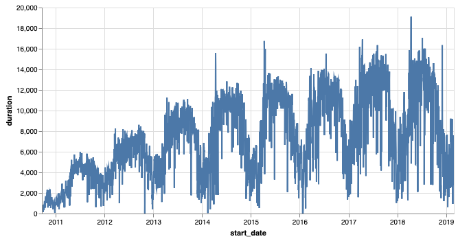
Let’s dive in and take a look at a graph of daily bike rentals.

Daily bike rentals for all days from Sept. 2010 through Feb. 2019.
Creating this graph is very easy if we use the Pandas resample method, which
works with timestamp data. This is a much nicer way to work with time-series
data than breaking the date into columns for year, month, day, hour, minute,
etc. then using the groupby method on a list of columns. The resample
method allows us to calculate lots of summary information on many interesting
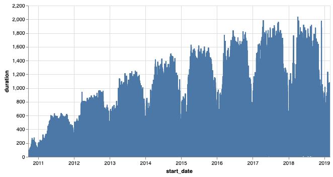
time scales. For example, we could look at rentals by the hour, but as you can see,
that is so dense that it’s pretty useless.

Hourly bike rentals for all days from Sept. 2010 through Feb. 2019.
The resample method takes several parameters, but the important one is the
one that specifies how you want it to resample. There are several options, and
here are the most common choices.
Parameter |
Description |
|---|---|
B |
Business day |
D |
Calendar day |
W |
Weekly |
M |
Month end |
Q |
Quarter end |
A |
Year end |
H |
Hourly |
T |
Minutely |
S |
Secondly |
The python code required to draw the daily graph is as follows.
resamp = trip_data.set_index('start_date')
resamp = resamp.resample('D').count()
resamp = resamp.reset_index()
Chart(resamp, width=600).mark_line().encode(
    x='start_date', y='duration').interactive()
First, we create a new DataFrame using the start_date as the index. This makes
it easier for us to work with the resample method and prepare for graphing.
Next, we call resamp.resample('D').count(). The 'D' parameter indicates
that we want to aggregate all of the rides for the day together and count the
number of rides each day. In addition, you can use mean, min,
max, median, and sum just like you have with groupby.
In order to graph the data with Altair, we need to make the index into a normal
column again. We reset the index and then draw the chart. The choice of
y='duration' is arbitrary.
| start_date | duration | end_date | start_station | end_station | bike_number | member_type | |
|---|---|---|---|---|---|---|---|
| 0 | 2010-09-20 | 212 | 212 | 212 | 212 | 212 | 212 |
| 1 | 2010-09-21 | 324 | 324 | 324 | 324 | 324 | 324 |
| 2 | 2010-09-22 | 377 | 377 | 377 | 377 | 377 | 377 |
| 3 | 2010-09-23 | 373 | 373 | 373 | 373 | 373 | 373 |
| 4 | 2010-09-24 | 362 | 362 | 362 | 362 | 362 | 362 |
Experiment with some resampling and graphing of the data. Try to graph by business day and week, instead of day, to get an idea.
Graph the mean ride length on a daily scale. Do you notice any trends in terms of days that have longer or shorter rides? Make a graph that overlays all days of the week with just the business days.
If you zoom in on the spikes and consult a calendar, you will see that it looks like Sunday is a winner for longer bike rides.
resamp = trip_data[trip_data.start_date < '2012-01-01'].set_index('start_date')
resamp = resamp.resample('D').mean()
resamp = resamp.reset_index()
d = Chart(resamp, width=600).mark_line().encode(
    x='start_date',y='duration').interactive()
resamp = trip_data[trip_data.start_date < '2012-01-01'].set_index('start_date')
resamp = resamp.resample('B').mean()
resamp = resamp.reset_index()
b = Chart(resamp, width=600).mark_line(color='red').encode(
    x='start_date',y='duration').interactive()
d+b
9.11.1. Indexing with a DatetimeIndex
Using a timestamp as an index gives you some additional power. For example, you
can use the index to select a year: resamp['2010'] will return all rows for
the year 2010, while resamp['2010-10'] will return all the rows for the
month of October in 2010. This gives you incredible power and flexibility for
working with date-indexed data.
9.11.2. Next Step: Predicting Rentals
Let’s take another look at the graph of bike rentals.

Daily bike rentals for all days from Sept. 2010 through Feb. 2019.
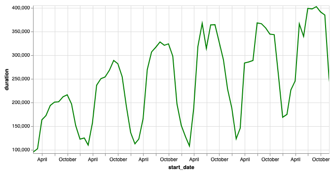
This graph indicates there is an overall upward trend in bike rentals in the DC area. Although it looks like it might be starting to level off in the 2017-2018 time frame. Within that overall trend of growth, we can see that there are seasonal variations as well as daily variations.

Seasonal variation in bike rentals
A time-series graph like this is very similar to a graph of airline travel, stock prices, and others. In the next few sections, we are going to try to develop a model that will allow us to predict the number of bike rentals on a particular day. There are many ways that we can do this, but one of the most common models to start with for making predictions is “linear regression”. But first, let’s take a break for some pizza.
9.11.3. Working with ZIP Files (Optional)
In many cases, large data files are available in compressed format. Usually, this is either ZIP or gzip format. Python allows us to work with the ZIP files directly so we don’t have to manually uncompress and recompress the files just to save disk space. This example shows you how to create a DataFrame of all the bike share data, using the assumption that you have downloaded all the files you need into a folder, and have no other files in that folder.
from zipfile import ZipFile
import os

bdfs = []
zipfiles = os.listdir('../Data/bikeshare')
for f in zipfiles:
    with ZipFile(f'../Data/bikeshare/{f}') as myzip:
        for zf in myzip.namelist():
            print(zf)
            if zf[-3:] == 'csv' and not zf[:2] == '__':
                with myzip.open(zf) as ridedata:
                    t = pd.read_csv(ridedata,
                                    parse_dates=['Start date', 'End date'])
                    t.columns = list(cmap.values())
                    t = t.drop(['start_location', 'end_location'], axis=1)
                    bdfs.append(t)

trip_data = pd.concat(bdfs)
The os.listdir call on line 5 looks at the directory and returns a list
containing all the filenames of files there. The with ZipFile... line opens
the .zip file as an object that you can manipulate. In particular, we would
like to be able to find out all the files that have been compressed and stored
in our zip, and we would like to be able to open them just like any other file.
Except that when we use myzip.open on line 12, Python will automatically
uncompress the file for us. The rest of the lines simply use pd.read_csv to read
in the uncompressed data, create a DataFrame, and store that DataFrame in a list
for us to use when we use pd.concat to concatenate all of the DataFrames
into a single large DataFrame.
Lesson Feedback
-
During this lesson I was primarily in my...
- 1. Comfort Zone
- 2. Learning Zone
- 3. Panic Zone
-
Completing this lesson took...
- 1. Very little time
- 2. A reasonable amount of time
- 3. More time than is reasonable
-
Based on my own interests and needs, the things taught in this lesson...
- 1. Don't seem worth learning
- 2. May be worth learning
- 3. Are definitely worth learning
-
For me to master the things taught in this lesson feels...
- 1. Definitely within reach
- 2. Within reach if I try my hardest
- 3. Out of reach no matter how hard I try