4.8. Probability of Connectivity

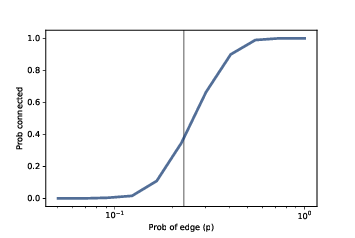
Figure 4.5: Probability of connectivity with n=10 and a range of p. The vertical line shows the predicted critical value.

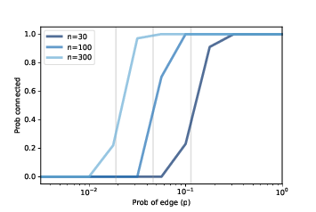
Figure 4.6: Probability of connectivity for several values of n and a range of p.

For given values of $n$ and $p$, we would like to know the probability that $G(n,p)$ is connected. We can estimate it by generating a large number of random graphs and counting how many are connected. Here’s how:

def prob_connected(n, p, iters=100):
tf = [is_connected(make_random_graph(n, p))
      for i in range(iters)]
return np.mean(bool)

The parameters n and p are passed along to make_random_graph; iters is the number of random graphs we generate.

The result, tf, is a list of boolean values: True for each graph that’s connected and False for each one that’s not.

np.mean is a NumPy function that computes the mean of this list, treating True as 1 and False as 0. The result is the fraction of random graphs that are connected.

>>> prob_connected(10, 0.23, iters=10000)
0.33

We chose 0.23 because it is close to the critical value where the probability of connectivity goes from near 0 to near 1. According to Erdős and Rényi, $p\ast =lnn/n=0.23$.

We can get a clearer view of the transition by estimating the probability of connectivity for a range of values of $p$:

n = 10
ps = np.logspace(-2.5, 0, 11)
ys = [prob_connected(n, p) for p in ps]

The NumPy function logspace returns an array of $11$ values from ${10}^{-2.5}$ to ${10}^0=1$, equally spaced on a logarithmic scale.

For each value of p in the array, we compute the probability that a graph with parameter p is connected and store the results in ys.

Figure 4.5 shows the results, with a vertical line at the computed critical value, $p\ast =0.23$. As expected, the transition from 0 to 1 occurs near the critical value.

Figure 4.6 shows similar results for larger values of n. As n increases, the critical value gets smaller and the transition gets more abrupt.

These experimental results are consistent with the analytic results Erdős and Rényi presented in their papers.

You have attempted 1 of 1 activities on this page